Section 7.1: Estimation
Section 7.1.1: Unbiasedness and Consistency
## simulation parameters
n <- 100 # sample size
mu0 <- 0 # mean of Y_i(0)
sd0 <- 1 # standard deviation of Y_i(0)
mu1 <- 1 # mean of Y_i(1)
sd1 <- 1 # standard deviation of Y_i(1)

## generate a sample
Y0 <- rnorm(n, mean = mu0, sd = sd0)
Y1 <- rnorm(n, mean = mu1, sd = sd1)
tau <- Y1 - Y0 # individual treatment effect
## true value of the sample average treatment effect
SATE <- mean(tau)
SATE
## [1] 0.7910608
## repeatedly conduct randomized controlled trials
sims <- 5000 # repeat 5,000 times, we could do more
diff.means <- rep(NA, sims)  # container

for (i in 1:sims) {
    ## randomize the treatment by sampling of a vector of 0's and 1's
    treat <- sample(c(rep(1, n / 2), rep(0, n / 2)), size = n, replace = FALSE)
    ## difference-in-means
    diff.means[i] <- mean(Y1[treat == 1]) - mean(Y0[treat == 0])
}

## estimation error for SATE
est.error <- diff.means - SATE
summary(est.error)
##      Min.   1st Qu.    Median      Mean   3rd Qu.      Max.
## -0.542364 -0.104843  0.005036  0.002633  0.114995  0.569677
## PATE simulation
PATE <- mu1 - mu0
diff.means <- rep(NA, sims)
for (i in 1:sims) {
    ## generate a sample for each simulation: this used to be outside of loop
    Y0 <- rnorm(n, mean = mu0, sd = sd0)
    Y1 <- rnorm(n, mean = mu1, sd = sd1)
    treat <- sample(c(rep(1, n / 2), rep(0, n / 2)), size = n, replace = FALSE)
    diff.means[i] <- mean(Y1[treat == 1]) - mean(Y0[treat == 0])
}

## estimation error for PATE
est.error <- diff.means - PATE

## unbiased
summary(est.error)
##       Min.    1st Qu.     Median       Mean    3rd Qu.       Max.
## -0.6947626 -0.1348674 -0.0024725  0.0000347  0.1324152  0.7546195
Section 7.1.2: Standard Error
par(cex = 1.5)
hist(diff.means, freq = FALSE, xlab = "Difference-in-means estimator",
     main = "Sampling distribution")
abline(v = SATE, col = "red") # true value of SATE
text(0.6, 2.4, "true SATE", col = "red")
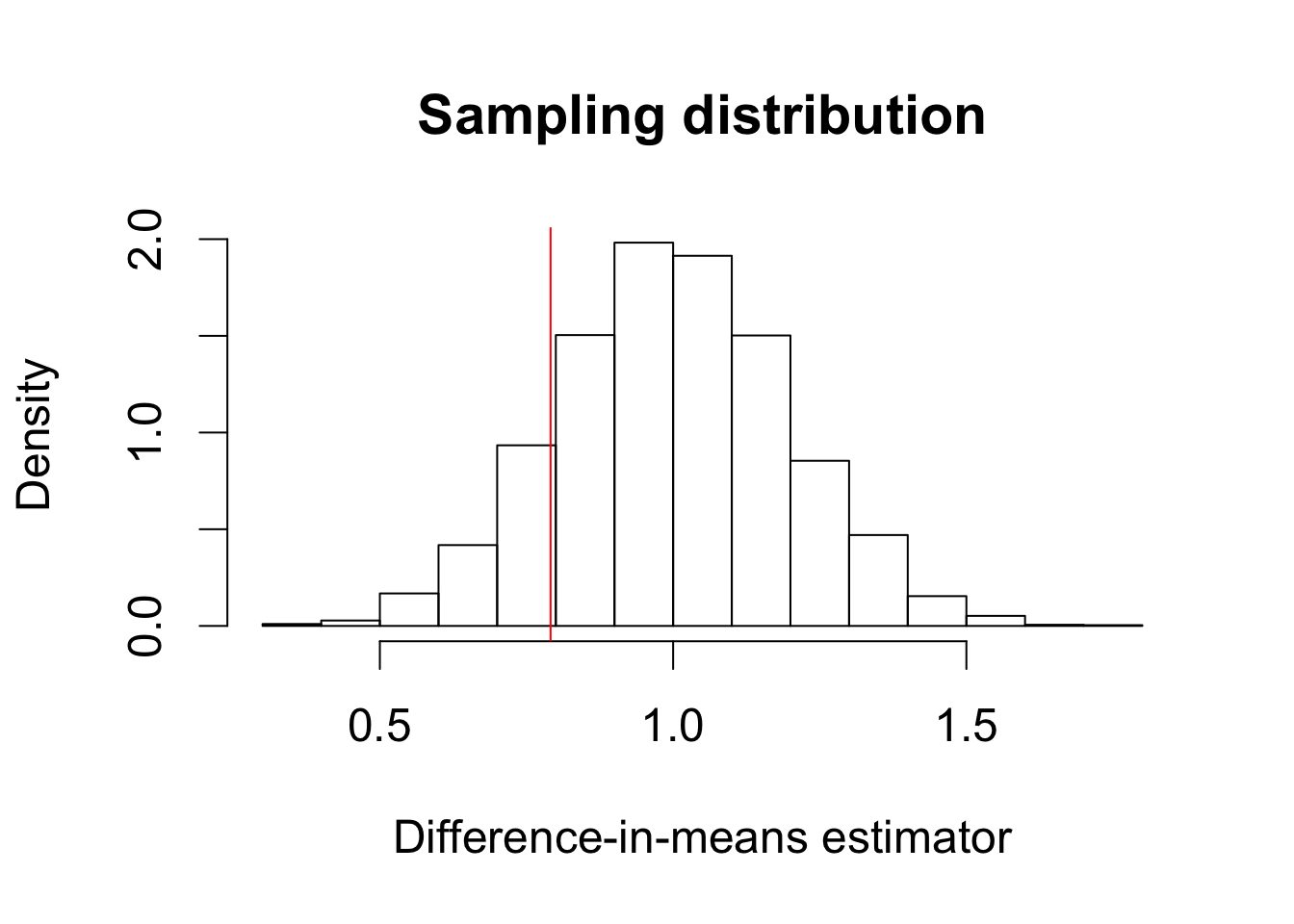
sd(diff.means)
## [1] 0.1973403
sqrt(mean((diff.means - SATE)^2))
## [1] 0.2874117
## PATE simulation with standard error
sims <- 5000
diff.means <- se <- rep(NA, sims)  # container for standard error added
for (i in 1:sims) {
    ## generate a sample
    Y0 <- rnorm(n, mean = mu0, sd = sd0)
    Y1 <- rnorm(n, mean = mu1, sd = sd1)
    ## randomize the treatment by sampling of a vector of 0's and 1's
    treat <- sample(c(rep(1, n / 2), rep(0, n / 2)), size = n, replace = FALSE)
    diff.means[i] <- mean(Y1[treat == 1]) - mean(Y0[treat == 0])
    ## standard error
    se[i] <- sqrt(var(Y1[treat == 1]) / (n / 2) + var(Y0[treat == 0]) / (n / 2))
}

## standard deviation of difference-in-means
sd(diff.means)
## [1] 0.2006359
## mean of standard errors
mean(se)
## [1] 0.199848
Section 7.1.3: Confidence Intervals
n <- 1000 # sample size
x.bar <- 0.6 # point estimate
s.e. <- sqrt(x.bar * (1 - x.bar) / n) # standard error
## 99% confidence intervals
c(x.bar - qnorm(0.995) * s.e., x.bar + qnorm(0.995) * s.e.)
## [1] 0.5600954 0.6399046
## 95% confidence intervals
c(x.bar - qnorm(0.975) * s.e., x.bar + qnorm(0.975) * s.e.)
## [1] 0.5696364 0.6303636
## 90% confidence intervals
c(x.bar - qnorm(0.95) * s.e., x.bar + qnorm(0.95) * s.e.)
## [1] 0.574518 0.625482
## empty container matrices for 2 sets of confidence intervals
ci95 <- ci90 <- matrix(NA, ncol = 2, nrow = sims)
## 95 percent confidence intervals
ci95[, 1] <- diff.means - qnorm(0.975) * se # lower limit
ci95[, 2] <- diff.means + qnorm(0.975) * se # upper limit

## 90 percent confidence intervals
ci90[, 1] <- diff.means - qnorm(0.95) * se # lower limit
ci90[, 2] <- diff.means + qnorm(0.95) * se # upper limit

## coverage rate for 95% confidence interval
mean(ci95[, 1] <= 1 & ci95[, 2] >= 1)
## [1] 0.9452
## coverage rate for 90% confidence interval
mean(ci90[, 1] <= 1 & ci90[, 2] >= 1)
## [1] 0.895
p <- 0.6 # true parameter value
n <- c(50, 100, 1000) # 3 sample sizes to be examined
alpha <- 0.05
sims <- 5000 # number of simulations
results <- rep(NA, length(n)) # a container for results

## loop for different sample sizes
for (i in 1:length(n)) {
    ci.results <- rep(NA, sims) # a container for whether CI includes truth
    ## loop for repeated hypothetical survey sampling
    for (j in 1:sims) {
        data <- rbinom(n[i], size = 1, prob = p) # simple random sampling
        x.bar <- mean(data) # sample proportion as an estimate
        s.e. <- sqrt(x.bar * (1 - x.bar) / n[i]) # standard errors
        ci.lower <- x.bar - qnorm(1 - alpha/2) * s.e.
        ci.upper <- x.bar + qnorm(1 - alpha/2) * s.e.
        ci.results[j] <- (p >= ci.lower) & (p <= ci.upper)
    }
    ## proportion of CIs that contain the true value
    results[i] <- mean(ci.results)
}
results
## [1] 0.9398 0.9516 0.9464
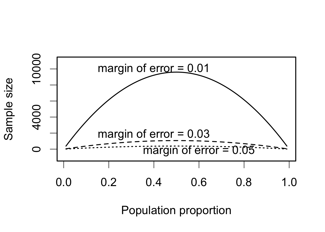
Scetion 7.1.4: Margin of Error and Sample Size Calculation in Polls
par(cex = 1.5, lwd = 2)
MoE <- c(0.01, 0.03, 0.05)  # the desired margin of error
p <- seq(from = 0.01, to = 0.99, by = 0.01)
n <- 1.96^2 * p * (1 - p) / MoE[1]^2
plot(p, n, ylim = c(-1000, 11000), xlab = "Population proportion",
     ylab = "Sample size", type = "l")
lines(p, 1.96^2 * p * (1 - p) / MoE[2]^2, lty = "dashed")
lines(p, 1.96^2 * p * (1 - p) / MoE[3]^2, lty = "dotted")
text(0.4, 10000, "margin of error = 0.01")
text(0.4, 1800, "margin of error = 0.03")
text(0.6, -200, "margin of error = 0.05")
## election and polling results, by state
data("pres08", package = "qss")
data("polls08", package = "qss")

## convert to a Date object
polls08$middate <- as.Date(polls08$middate)
## number of days to the election day
polls08$DaysToElection <- as.Date("2008-11-04") - polls08$middate
## Warning in strptime(xx, f <- "%Y-%m-%d", tz = "GMT"): unknown timezone
## 'zone/tz/2017c.1.0/zoneinfo/America/New_York'
## create a matrix place holder
poll.pred <- matrix(NA, nrow = 51, ncol = 3)

## state names which the loop will iterate through
st.names <- unique(pres08$state)
## add labels for easy interpretation later on
row.names(poll.pred) <- as.character(st.names)

## loop across 50 states plus DC
for (i in 1:51){
    ## subset the ith state
    state.data <- subset(polls08, subset = (state == st.names[i]))
    ## subset the latest polls within the state
    latest <- state.data$DaysToElection == min(state.data$DaysToElection)
    ## compute the mean of latest polls and store it
    poll.pred[i, 1] <- mean(state.data$Obama[latest]) / 100
}

## upper and lower confidence limits
n <- 1000 # sample size
alpha <- 0.05
s.e. <- sqrt(poll.pred[, 1] * (1 - poll.pred[, 1]) / n) # standard error
poll.pred[, 2] <- poll.pred[, 1] - qnorm(1 - alpha/2) * s.e.
poll.pred[, 3] <- poll.pred[, 1] + qnorm(1 - alpha/2) * s.e.

par(cex = 1.5)
alpha <- 0.05
plot(pres08$Obama / 100, poll.pred[, 1], xlim = c(0, 1), ylim = c(0, 1),
     xlab = "Obama's vote share", ylab = "Poll prediction")
abline(0, 1)

## adding 95% confidence intervals for each state
for (i in 1:51) {
    lines(rep(pres08$Obama[i] / 100, 2), c(poll.pred[i, 2], poll.pred[i, 3]))
}
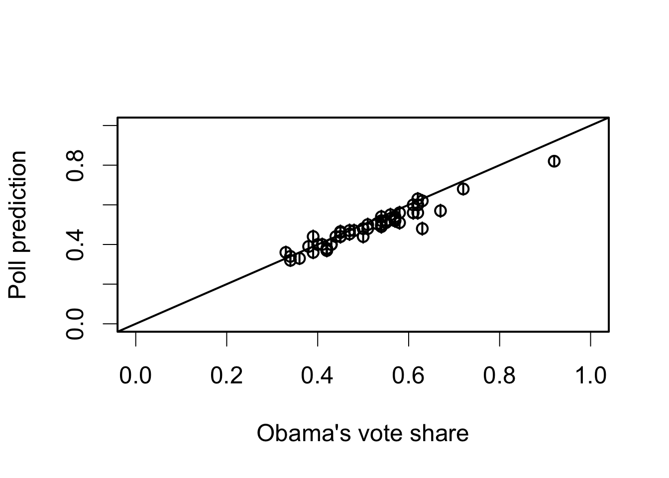
## proportion of confidence intervals that contain the election day outcome
mean((poll.pred[, 2] <= pres08$Obama / 100) &
         (poll.pred[, 3] >= pres08$Obama / 100))
## [1] 0.5882353
## bias
bias <- mean(poll.pred[, 1] - pres08$Obama / 100)
bias
## [1] -0.02679739
## bias corrected estimate
poll.bias <- poll.pred[, 1] - bias
## bias-corrected standard error
s.e.bias <- sqrt(poll.bias * (1 - poll.bias) / n)
## bias-corrected 95% confidence interval
ci.bias.lower <- poll.bias - qnorm(1 - alpha / 2) * s.e.bias
ci.bias.upper <- poll.bias + qnorm(1 - alpha / 2) * s.e.bias

## proportion of bias-corrected CIs that contain the election day outcome
mean((ci.bias.lower <= pres08$Obama / 100) &
         (ci.bias.upper >= pres08$Obama / 100))
## [1] 0.7647059
Section 7.1.5: Analysis of Randomized Controlled Trials
par(cex = 1.5)
## read in data
data("STAR", package = "qss")
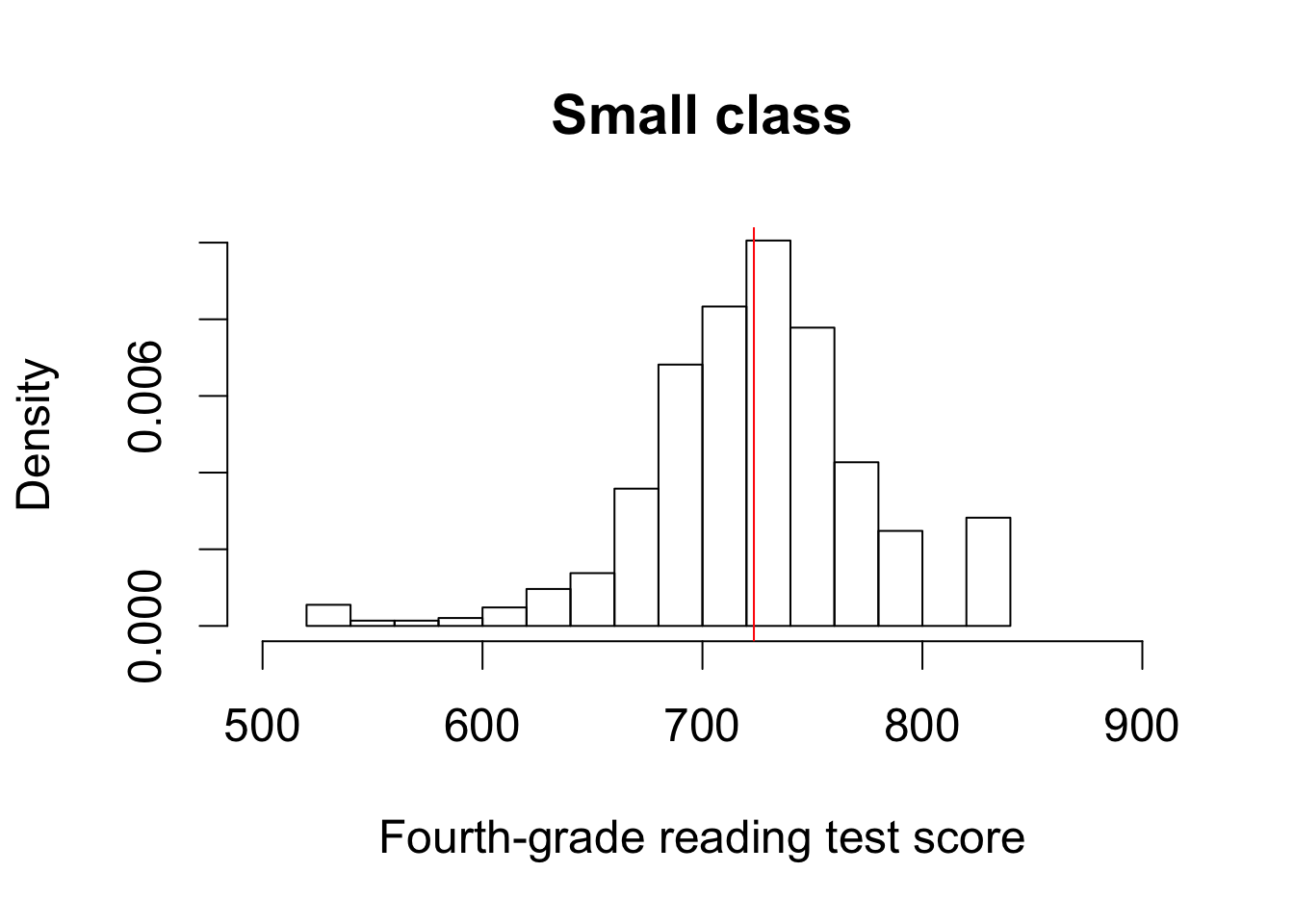
hist(STAR$g4reading[STAR$classtype == 1], freq = FALSE, xlim = c(500, 900),
ylim = c(0, 0.01), main = "Small class",
xlab = "Fourth-grade reading test score")
abline(v = mean(STAR$g4reading[STAR$classtype == 1], na.rm = TRUE),
col = "red")
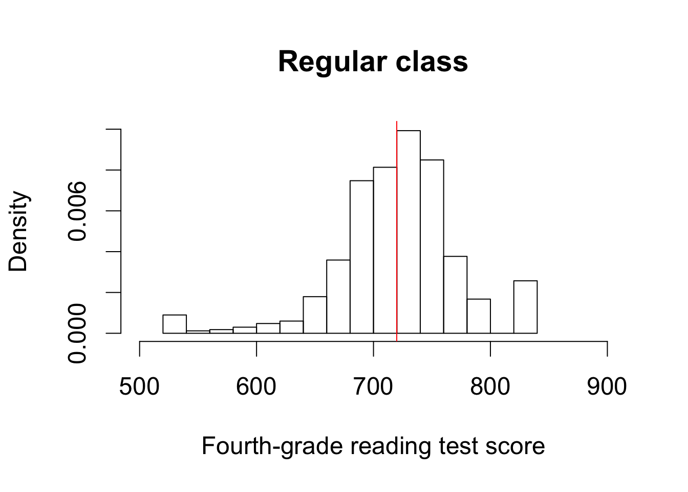
hist(STAR$g4reading[STAR$classtype == 2], freq = FALSE, xlim = c(500, 900),
     ylim = c(0, 0.01), main = "Regular class",
     xlab = "Fourth-grade reading test score")
abline(v = mean(STAR$g4reading[STAR$classtype == 2], na.rm = TRUE),
       col = "red")
## estimate and standard error for small class
n.small <- sum(STAR$classtype == 1 & !is.na(STAR$g4reading))
est.small <- mean(STAR$g4reading[STAR$classtype == 1], na.rm = TRUE)
se.small <- sd(STAR$g4reading[STAR$classtype == 1], na.rm = TRUE) /
    sqrt(n.small)
est.small
## [1] 723.3912
se.small
## [1] 1.913012
## estimate and standard error for regular class
n.regular <- sum(STAR$classtype == 2 & !is.na(STAR$classtype) &
                     !is.na(STAR$g4reading))
est.regular <- mean(STAR$g4reading[STAR$classtype == 2], na.rm = TRUE)
se.regular <- sd(STAR$g4reading[STAR$classtype == 2], na.rm = TRUE) /
    sqrt(n.regular)
est.regular
## [1] 719.89
se.regular
## [1] 1.83885
alpha <- 0.05
## 95% confidence intervals for small class
ci.small <- c(est.small - qnorm(1 - alpha / 2) * se.small,
              est.small + qnorm(1 - alpha / 2) * se.small)
ci.small
## [1] 719.6417 727.1406
## 95% confidence intervals for regular class
ci.regular <- c(est.regular - qnorm(1 - alpha / 2) * se.regular,
                est.regular + qnorm(1 - alpha / 2) * se.regular)
ci.regular
## [1] 716.2859 723.4940
## difference-in-means estimator
ate.est <- est.small - est.regular
ate.est
## [1] 3.501232
## standard error and 95% confidence interval
ate.se <- sqrt(se.small^2 + se.regular^2)
ate.se
## [1] 2.653485
ate.ci <- c(ate.est - qnorm(1 - alpha / 2) * ate.se,
            ate.est + qnorm(1 - alpha / 2) * ate.se)
ate.ci
## [1] -1.699503 8.701968
Section 7.1.6: Analysis Based on Student’s t-Distribution
## 95% CI for small class
c(est.small - qt(0.975, df = n.small - 1) * se.small,
  est.small + qt(0.975, df = n.small - 1) * se.small)
## [1] 719.6355 727.1469
## 95% CI based on the central limit theorem
ci.small
## [1] 719.6417 727.1406
## 95% CI for regular class
c(est.regular - qt(0.975, df = n.regular - 1) * se.regular,
  est.regular + qt(0.975, df = n.regular - 1) * se.regular)
## [1] 716.2806 723.4993
## 95% CI based on the central limit theorem
ci.regular
## [1] 716.2859 723.4940
t.ci <- t.test(STAR$g4reading[STAR$classtype == 1],
               STAR$g4reading[STAR$classtype == 2])
t.ci
##
##  Welch Two Sample t-test
##
## data:  STAR$g4reading[STAR$classtype == 1] and STAR$g4reading[STAR$classtype == 2]
## t = 1.3195, df = 1541.2, p-value = 0.1872
## alternative hypothesis: true difference in means is not equal to 0
## 95 percent confidence interval:
##  -1.703591  8.706055
## sample estimates:
## mean of x mean of y
##  723.3912  719.8900
Section 7.2: Hypothesis Testing
Section 7.2.1: Tea-Testing Experiment
## truth: enumerate the number of assignment combinations
true <- c(choose(4, 0) * choose(4, 4),
          choose(4, 1) * choose(4, 3),
          choose(4, 2) * choose(4, 2),
          choose(4, 3) * choose(4, 1),
          choose(4, 4) * choose(4, 0))
true
## [1] 1 16 36 16 1
## compute probability: divide it by the total number of events
true <- true / sum(true)
## number of correctly classified cups as labels
names(true) <- c(0, 2, 4, 6, 8)
true
##          0          2          4          6          8
## 0.01428571 0.22857143 0.51428571 0.22857143 0.01428571
## simulations
sims <- 1000
## lady's guess: M stands for `Milk first,' T stands for `Tea first'
guess <- c("M", "T", "T", "M", "M", "T", "T", "M")
correct <- rep(NA, sims) # place holder for number of correct guesses
for (i in 1:sims) {
    ## randomize which cups get Milk/Tea first
    cups <- sample(c(rep("T", 4), rep("M", 4)), replace = FALSE)
    correct[i] <- sum(guess == cups) # number of correct guesses
}
## estimated probability for each number of correct guesses
prop.table(table(correct))
## correct
##     0     2     4     6     8
## 0.017 0.227 0.506 0.238 0.012
## comparison with analytical answers; the differences are small
prop.table(table(correct)) - true
## correct
##            0            2            4            6            8
##  0.002714286 -0.001571429 -0.008285714  0.009428571 -0.002285714
Section 7.2.2: The General Framework
## all correct
x <- matrix(c(4, 0, 0, 4), byrow = TRUE, ncol = 2, nrow = 2)
## six correct
y <- matrix(c(3, 1, 1, 3), byrow = TRUE, ncol = 2, nrow = 2)

## `M' milk first, `T' tea first
rownames(x) <- colnames(x) <- rownames(y) <- colnames(y) <- c("M", "T")
x
##   M T
## M 4 0
## T 0 4
y
##   M T
## M 3 1
## T 1 3
## one-sided test for 8 correct guesses
fisher.test(x, alternative = "greater")
##
##  Fisher's Exact Test for Count Data
##
## data:  x
## p-value = 0.01429
## alternative hypothesis: true odds ratio is greater than 1
## 95 percent confidence interval:
##  2.003768      Inf
## sample estimates:
## odds ratio
##        Inf
## two-sided test for 6 correct guesses
fisher.test(y)
##
##  Fisher's Exact Test for Count Data
##
## data:  y
## p-value = 0.4857
## alternative hypothesis: true odds ratio is not equal to 1
## 95 percent confidence interval:
##    0.2117329 621.9337505
## sample estimates:
## odds ratio
##   6.408309
Section 7.2.3: One-Sample Tests
n <- 1018
x.bar <- 550 / n
se <- sqrt(0.5 * 0.5 / n) # standard deviation of sampling distribution

## upper red area in the figure
upper <- pnorm(x.bar, mean = 0.5, sd = se, lower.tail = FALSE)

## lower red area in the figure; identical to the upper area
lower <- pnorm(0.5 - (x.bar - 0.5), mean = 0.5, sd = se)

## two-side p-value
upper + lower
## [1] 0.01016866
2 * upper
## [1] 0.01016866
## one-sided p-value
upper
## [1] 0.005084332
z.score <- (x.bar - 0.5) / se
z.score
## [1] 2.57004
pnorm(z.score, lower.tail = FALSE) # one-sided p-value
## [1] 0.005084332
2 * pnorm(z.score, lower.tail = FALSE) # two-sided p-value
## [1] 0.01016866
## 99% confidence interval contains 0.5
c(x.bar - qnorm(0.995) * se, x.bar + qnorm(0.995) * se)
## [1] 0.4999093 0.5806408
## 95% confidence interval does not contain 0.5
c(x.bar - qnorm(0.975) * se, x.bar + qnorm(0.975) * se)
## [1] 0.5095605 0.5709896
## no continuity correction to get the same p-value as above
prop.test(550, n = n, p = 0.5, correct = FALSE)
##
##  1-sample proportions test without continuity correction
##
## data:  550 out of n, null probability 0.5
## X-squared = 6.6051, df = 1, p-value = 0.01017
## alternative hypothesis: true p is not equal to 0.5
## 95 percent confidence interval:
##  0.5095661 0.5706812
## sample estimates:
##        p
## 0.540275
## with continuity correction
prop.test(550, n = n, p = 0.5)
##
##  1-sample proportions test with continuity correction
##
## data:  550 out of n, null probability 0.5
## X-squared = 6.445, df = 1, p-value = 0.01113
## alternative hypothesis: true p is not equal to 0.5
## 95 percent confidence interval:
##  0.5090744 0.5711680
## sample estimates:
##        p
## 0.540275
prop.test(550, n = n, p = 0.5, conf.level = 0.99)
##
##  1-sample proportions test with continuity correction
##
## data:  550 out of n, null probability 0.5
## X-squared = 6.445, df = 1, p-value = 0.01113
## alternative hypothesis: true p is not equal to 0.5
## 99 percent confidence interval:
##  0.4994182 0.5806040
## sample estimates:
##        p
## 0.540275
## two-sided one-sample t-test
t.test(STAR$g4reading, mu = 710)
##
##  One Sample t-test
##
## data:  STAR$g4reading
## t = 10.407, df = 2352, p-value < 2.2e-16
## alternative hypothesis: true mean is not equal to 710
## 95 percent confidence interval:
##  719.1284 723.3671
## sample estimates:
## mean of x
##  721.2478
Section 7.2.4: Two-Sample Tests
## one-sided p-value
pnorm(-abs(ate.est), mean = 0, sd = ate.se)
## [1] 0.09350361
## two-sided p-value
2 * pnorm(-abs(ate.est), mean = 0, sd = ate.se)
## [1] 0.1870072
## testing the null of zero average treatment effect
t.test(STAR$g4reading[STAR$classtype == 1],
       STAR$g4reading[STAR$classtype == 2])
##
##  Welch Two Sample t-test
##
## data:  STAR$g4reading[STAR$classtype == 1] and STAR$g4reading[STAR$classtype == 2]
## t = 1.3195, df = 1541.2, p-value = 0.1872
## alternative hypothesis: true difference in means is not equal to 0
## 95 percent confidence interval:
##  -1.703591  8.706055
## sample estimates:
## mean of x mean of y
##  723.3912  719.8900
data("resume", package = "qss")

## organize the data in tables
x <- table(resume$race, resume$call)
x
##
##            0    1
##   black 2278  157
##   white 2200  235
## one-sided test
prop.test(x, alternative = "greater")
##
##  2-sample test for equality of proportions with continuity
##  correction
##
## data:  x
## X-squared = 16.449, df = 1, p-value = 2.499e-05
## alternative hypothesis: greater
## 95 percent confidence interval:
##  0.01881967 1.00000000
## sample estimates:
##    prop 1    prop 2
## 0.9355236 0.9034908
## sample size
n0 <- sum(resume$race == "black")
n1 <- sum(resume$race == "white")

## sample proportions
p <- mean(resume$call) # overall
p0 <- mean(resume$call[resume$race == "black"]) # black
p1 <- mean(resume$call[resume$race == "white"]) # white

## point estimate
est <- p1 - p0
est
## [1] 0.03203285
## standard error
se <- sqrt(p * (1 - p) * (1 / n0 + 1 / n1))
se
## [1] 0.007796894
## z-statistic
zstat <- est / se
zstat
## [1] 4.108412
## one-sided p-value
pnorm(-abs(zstat))
## [1] 1.991943e-05
prop.test(x, alternative = "greater", correct = FALSE)
##
##  2-sample test for equality of proportions without continuity
##  correction
##
## data:  x
## X-squared = 16.879, df = 1, p-value = 1.992e-05
## alternative hypothesis: greater
## 95 percent confidence interval:
##  0.01923035 1.00000000
## sample estimates:
##    prop 1    prop 2
## 0.9355236 0.9034908
Section 7.2.5: Pitfalls of Hypothesis Testing
Section 7.2.6: Power Analysis
## set the parameters
n <- 250
p.star <- 0.48 # data generating process
p <- 0.5 # null value
alpha <- 0.05

## critical value
cr.value <- qnorm(1 - alpha / 2)

## standard errors under the hypothetical data generating process
se.star <- sqrt(p.star * (1 - p.star) / n)

## standard error under the null
se <- sqrt(p * (1 - p) / n)

## power
pnorm(p - cr.value * se, mean = p.star, sd = se.star) +
    pnorm(p + cr.value * se, mean = p.star, sd = se.star, lower.tail = FALSE)
## [1] 0.09673114
## parameters
n1 <- 500
n0 <- 500
p1.star <- 0.05
p0.star <- 0.1

## overall call back rate as a weighted average
p <- (n1 * p1.star + n0 * p0.star) / (n1 + n0)
## standard error under the null
se <- sqrt(p * (1 - p) * (1 / n1 + 1 / n0))
## standard error under the hypothetical data generating process
se.star <- sqrt(p1.star * (1 - p1.star) / n1 + p0.star * (1 - p0.star) / n0)

pnorm(-cr.value * se, mean = p1.star - p0.star, sd = se.star) +
    pnorm(cr.value * se, mean = p1.star - p0.star, sd = se.star,
          lower.tail = FALSE)
## [1] 0.85228
power.prop.test(n = 500, p1 = 0.05, p2 = 0.1, sig.level = 0.05)
##
##      Two-sample comparison of proportions power calculation
##
##               n = 500
##              p1 = 0.05
##              p2 = 0.1
##       sig.level = 0.05
##           power = 0.8522797
##     alternative = two.sided
##
## NOTE: n is number in *each* group
power.prop.test(p1 = 0.05, p2 = 0.1, sig.level = 0.05, power = 0.9)
##
##      Two-sample comparison of proportions power calculation
##
##               n = 581.0821
##              p1 = 0.05
##              p2 = 0.1
##       sig.level = 0.05
##           power = 0.9
##     alternative = two.sided
##
## NOTE: n is number in *each* group
power.t.test(n = 100, delta = 0.25, sd = 1, type = "one.sample")
##
##      One-sample t test power calculation
##
##               n = 100
##           delta = 0.25
##              sd = 1
##       sig.level = 0.05
##           power = 0.6969757
##     alternative = two.sided
power.t.test(power = 0.9, delta = 0.25, sd = 1, type = "one.sample")
##
##      One-sample t test power calculation
##
##               n = 170.0511
##           delta = 0.25
##              sd = 1
##       sig.level = 0.05
##           power = 0.9
##     alternative = two.sided
power.t.test(delta = 0.25, sd = 1, type = "two.sample",
             alternative = "one.sided", power = 0.9)
##
##      Two-sample t test power calculation
##
##               n = 274.7222
##           delta = 0.25
##              sd = 1
##       sig.level = 0.05
##           power = 0.9
##     alternative = one.sided
##
## NOTE: n is number in *each* group
Section 7.3: Linear Regression Model with Uncertainty
Section 7.3.1: Linear Regression as a Generative Model
data("minwage", package = "qss")

## compute proportion of full employment before minimum wage increase
minwage$fullPropBefore <- minwage$fullBefore /
    (minwage$fullBefore + minwage$partBefore)

## same thing after minimum wage increase
minwage$fullPropAfter <- minwage$fullAfter /
    (minwage$fullAfter + minwage$partAfter)

## an indicator for NJ: 1 if it's located in NJ and 0 if in PA
minwage$NJ <- ifelse(minwage$location == "PA", 0, 1)

fit.minwage <- lm(fullPropAfter ~ -1 + NJ + fullPropBefore +
                      wageBefore + chain, data = minwage)

## regression result
fit.minwage
##
## Call:
## lm(formula = fullPropAfter ~ -1 + NJ + fullPropBefore + wageBefore +
##     chain, data = minwage)
##
## Coefficients:
##              NJ   fullPropBefore       wageBefore  chainburgerking
##         0.05422          0.16879          0.08133         -0.11563
##        chainkfc        chainroys      chainwendys
##        -0.15080         -0.20639         -0.22013
fit.minwage1 <- lm(fullPropAfter ~ NJ + fullPropBefore +
                       wageBefore + chain, data = minwage)
fit.minwage1
##
## Call:
## lm(formula = fullPropAfter ~ NJ + fullPropBefore + wageBefore +
##     chain, data = minwage)
##
## Coefficients:
##    (Intercept)              NJ  fullPropBefore      wageBefore
##       -0.11563         0.05422         0.16879         0.08133
##       chainkfc       chainroys     chainwendys
##       -0.03517        -0.09076        -0.10451
predict(fit.minwage, newdata = minwage[1, ])
##         1
## 0.2709367
predict(fit.minwage1, newdata = minwage[1, ])
##         1
## 0.2709367
Section 7.3.2: Unbiasedness of Estimated Coefficients
Section 7.3.3: Standard Errors of Estimated Coefficients
Section 7.3.4: Inference About Coefficients
data(women, package = "qss")
fit.women <- lm(water ~ reserved, data = women)
summary(fit.women)
##
## Call:
## lm(formula = water ~ reserved, data = women)
##
## Residuals:
##     Min      1Q  Median      3Q     Max
## -23.991 -14.738  -7.865   2.262 316.009
##
## Coefficients:
##             Estimate Std. Error t value Pr(>|t|)
## (Intercept)   14.738      2.286   6.446 4.22e-10 ***
## reserved       9.252      3.948   2.344   0.0197 *
## ---
## Signif. codes:  0 '***' 0.001 '**' 0.01 '*' 0.05 '.' 0.1 ' ' 1
##
## Residual standard error: 33.45 on 320 degrees of freedom
## Multiple R-squared:  0.01688,    Adjusted R-squared:  0.0138
## F-statistic: 5.493 on 1 and 320 DF,  p-value: 0.0197
confint(fit.women) # 95% confidence intervals
##                 2.5 %   97.5 %
## (Intercept) 10.240240 19.23640
## reserved     1.485608 17.01924
summary(fit.minwage)
##
## Call:
## lm(formula = fullPropAfter ~ -1 + NJ + fullPropBefore + wageBefore +
##     chain, data = minwage)
##
## Residuals:
##      Min       1Q   Median       3Q      Max
## -0.48617 -0.18135 -0.02809  0.15127  0.75091
##
## Coefficients:
##                 Estimate Std. Error t value Pr(>|t|)
## NJ               0.05422    0.03321   1.633  0.10343
## fullPropBefore   0.16879    0.05662   2.981  0.00307 **
## wageBefore       0.08133    0.03892   2.090  0.03737 *
## chainburgerking -0.11563    0.17888  -0.646  0.51844
## chainkfc        -0.15080    0.18310  -0.824  0.41074
## chainroys       -0.20639    0.18671  -1.105  0.26974
## chainwendys     -0.22013    0.18840  -1.168  0.24343
## ---
## Signif. codes:  0 '***' 0.001 '**' 0.01 '*' 0.05 '.' 0.1 ' ' 1
##
## Residual standard error: 0.2438 on 351 degrees of freedom
## Multiple R-squared:  0.6349, Adjusted R-squared:  0.6277
## F-statistic: 87.21 on 7 and 351 DF,  p-value: < 2.2e-16
## confidence interval just for the `NJ' variable
confint(fit.minwage)["NJ", ]
##       2.5 %      97.5 %
## -0.01109295  0.11953297
Section 7.3.5: Inference About Predictions
## load the data and subset them into two parties
data("MPs", package = "qss")
MPs.labour <- subset(MPs, subset = (party == "labour"))
MPs.tory <- subset(MPs, subset = (party == "tory"))
## two regressions for labour: negative and positive margin
labour.fit1 <- lm(ln.net ~ margin,
data = MPs.labour[MPs.labour$margin < 0, ])
labour.fit2 <- lm(ln.net ~ margin,
data = MPs.labour[MPs.labour$margin > 0, ])
## two regressions for tory: negative and positive margin
tory.fit1 <- lm(ln.net ~ margin, data = MPs.tory[MPs.tory$margin < 0, ])
tory.fit2 <- lm(ln.net ~ margin, data = MPs.tory[MPs.tory$margin > 0, ])
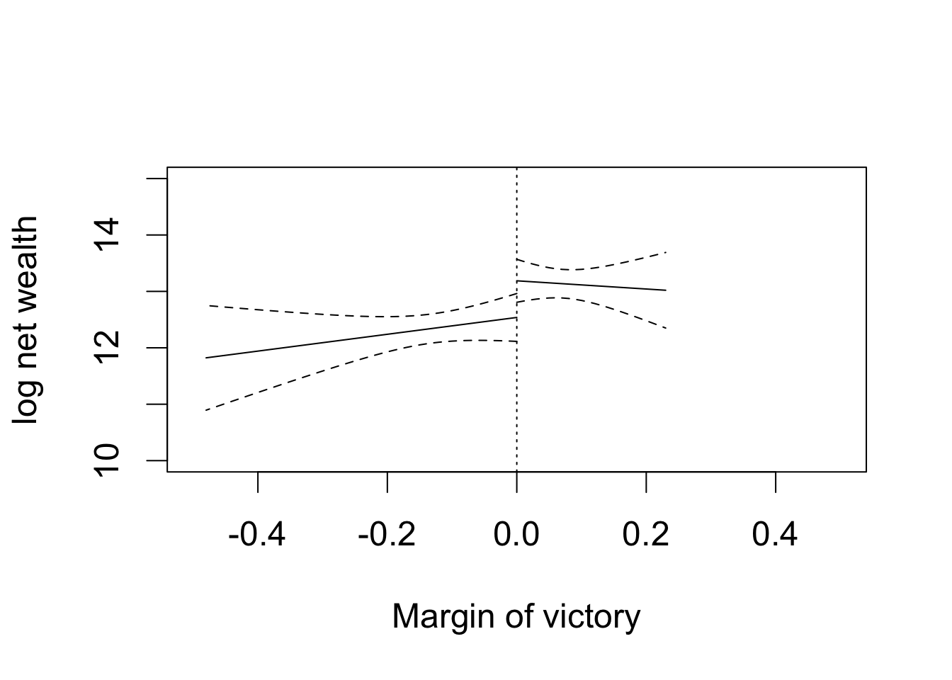
## tory party: prediction at the threshold
tory.y0 <- predict(tory.fit1, interval = "confidence",
newdata = data.frame(margin = 0))
tory.y0
##        fit      lwr      upr
## 1 12.53812 12.11402 12.96221
tory.y1 <- predict(tory.fit2, interval = "confidence",
                   newdata = data.frame(margin = 0))
tory.y1
##       fit      lwr      upr
## 1 13.1878 12.80691 13.56869
## range of predictors; min to 0 and 0 to max
y1.range <- seq(from = 0, to = min(MPs.tory$margin), by = -0.01)
y2.range <- seq(from = 0, to = max(MPs.tory$margin), by = 0.01)

## prediction using all the values
tory.y0 <- predict(tory.fit1, interval = "confidence",
                   newdata = data.frame(margin = y1.range))
tory.y1 <- predict(tory.fit2, interval = "confidence",
                   newdata = data.frame(margin = y2.range))

par(cex = 1.5)
## plotting the first regression with losers
plot(y1.range, tory.y0[, "fit"], type = "l", xlim = c(-0.5, 0.5),
     ylim = c(10, 15), xlab = "Margin of victory", ylab = "log net wealth")
abline(v = 0, lty = "dotted")
lines(y1.range, tory.y0[, "lwr"], lty = "dashed") # lower CI
lines(y1.range, tory.y0[, "upr"], lty = "dashed") # upper CI

## plotting the second regression with winners
lines(y2.range, tory.y1[, "fit"], lty = "solid")  # point estimates
lines(y2.range, tory.y1[, "lwr"], lty = "dashed") # lower CI
lines(y2.range, tory.y1[, "upr"], lty = "dashed") # upper CI
## re-compute the predicted value and return standard errors
tory.y0 <- predict(tory.fit1, interval = "confidence", se.fit = TRUE,
                   newdata = data.frame(margin = 0))
tory.y0
## $fit
##        fit      lwr      upr
## 1 12.53812 12.11402 12.96221
##
## $se.fit
## [1] 0.2141793
##
## $df
## [1] 119
##
## $residual.scale
## [1] 1.434283
tory.y1 <- predict(tory.fit2, interval = "confidence", se.fit = TRUE,
                   newdata = data.frame(margin = 0))

## s.e. of the intercept is the same as s.e. of the predicted value
summary(tory.fit1)
##
## Call:
## lm(formula = ln.net ~ margin, data = MPs.tory[MPs.tory$margin <
##     0, ])
##
## Residuals:
##     Min      1Q  Median      3Q     Max
## -5.3195 -0.4721 -0.0349  0.6629  3.5798
##
## Coefficients:
##             Estimate Std. Error t value Pr(>|t|)
## (Intercept)  12.5381     0.2142  58.540   <2e-16 ***
## margin        1.4911     1.2914   1.155    0.251
## ---
## Signif. codes:  0 '***' 0.001 '**' 0.01 '*' 0.05 '.' 0.1 ' ' 1
##
## Residual standard error: 1.434 on 119 degrees of freedom
## Multiple R-squared:  0.01108,    Adjusted R-squared:  0.002769
## F-statistic: 1.333 on 1 and 119 DF,  p-value: 0.2506
## standard error
se.diff <- sqrt(tory.y0$se.fit^2 + tory.y1$se.fit^2)
se.diff
## [1] 0.2876281
## point estimate
diff.est <- tory.y1$fit[1, "fit"] - tory.y0$fit[1, "fit"]
diff.est
## [1] 0.6496861
## confidence interval
CI <- c(diff.est - se.diff * qnorm(0.975), diff.est + se.diff * qnorm(0.975))
CI
## [1] 0.0859455 1.2134268
## hypothesis test
z.score <- diff.est / se.diff
p.value <- 2 * pnorm(abs(z.score), lower.tail = FALSE) # two-sided p-value
p.value
## [1] 0.02389759