Section 4.1: Predicting Election Outcomes
Section 4.1.1: Loops in R
values <- c(2, 4, 6)
n <- length(values) # number of elements in `values'
results <- rep(NA, n) # empty container vector for storing the results

## loop counter `i' will take values on 1, 2, ..., n in that order
for (i in 1:n) {
    ## store the result of multiplication as the ith element of
    ## `results' vector
    results[i] <- values[i] * 2
    cat(values[i], "times 2 is equal to", results[i], "\n")
}
## 2 times 2 is equal to 4
## 4 times 2 is equal to 8
## 6 times 2 is equal to 12
results
## [1] 4 8 12
## check if the code runs when i = 1
i <- 1
x <- values[i] * 2
cat(values[i], "times 2 is equal to", x, "\n")
## 2 times 2 is equal to 4
Section 4.1.2: General Conditional Statements in R
## define the operation to be executed
operation <- "add"
if (operation == "add") {
    cat("I will perform addition 4 + 4\n")
    4 + 4
}
## I will perform addition 4 + 4
## [1] 8
if (operation == "multiply") {
    cat("I will perform multiplication 4 * 4\n")
    4 * 4
}

## Note that `operation' is redefined
operation <- "multiply"
if (operation == "add") {
    cat("I will perform addition 4 + 4")
    4 + 4
} else {
    cat("I will perform multiplication 4 * 4")
    4 * 4
}
## I will perform multiplication 4 * 4
## [1] 16
## Note that `operation' is redefined
operation <- "subtract"
if (operation == "add") {
    cat("I will perform addition 4 + 4\n")
    4 + 4
} else if (operation == "multiply") {
    cat("I will perform multiplication 4 * 4\n")
    4 * 4
} else {
    cat("`", operation, "' is invalid. Use either `add' or `multiply'.\n",
        sep = "")
}
## `subtract' is invalid. Use either `add' or `multiply'.
values <- 1:5
n <-  length(values)
results <- rep(NA, n)
for (i in 1:n) {
    ## x and r get overwritten in each iteration
    x <- values[i]
    r <- x %% 2  # remainder when divided by 2 to check whether even or odd
    if (r == 0) { # remainder is zero
        cat(x, "is even and I will perform addition",
            x, "+", x, "\n")
        results[i] <- x + x
    } else { # remainder is not zero
        cat(x, "is odd and I will perform multiplication",
            x, "*", x, "\n")
        results[i] <- x * x
    }
}
## 1 is odd and I will perform multiplication 1 * 1
## 2 is even and I will perform addition 2 + 2
## 3 is odd and I will perform multiplication 3 * 3
## 4 is even and I will perform addition 4 + 4
## 5 is odd and I will perform multiplication 5 * 5
results
## [1] 1 4 9 8 25
Section 4.1.3: Poll Predictions
## load election results, by state
data("pres08", package = "qss")
## load polling data
data("polls08", package = "qss")
## compute Obama's margin
polls08$margin <- polls08$Obama - polls08$McCain
pres08$margin <- pres08$Obama - pres08$McCain

x <- as.Date("2008-11-04")
## Warning in strptime(xx, f <- "%Y-%m-%d", tz = "GMT"): unknown timezone
## 'zone/tz/2017c.1.0/zoneinfo/America/New_York'
y <- as.Date("2008/9/1")
x - y # number of days between 2008/9/1 and 11/4
## Time difference of 64 days
## convert to a Date object
polls08$middate <- as.Date(polls08$middate)
## computer the number of days to the election day
polls08$DaysToElection <- as.Date("2008-11-04") - polls08$middate
poll.pred <- rep(NA, 51) # initialize a vector place holder
## extract unique state names which the loop will iterate through
st.names <- unique(polls08$state)
## add state names as labels for easy interpretation later on
names(poll.pred) <- as.character(st.names)
## loop across 50 states plus DC
for (i in 1:51){
## subset the ith state
state.data <- subset(polls08, subset = (state == st.names[i]))
## further subset the latest polls within the state
latest <- subset(state.data, DaysToElection == min(DaysToElection))
## compute the mean of latest polls and store it
poll.pred[i] <- mean(latest$margin)
}
## error of latest polls
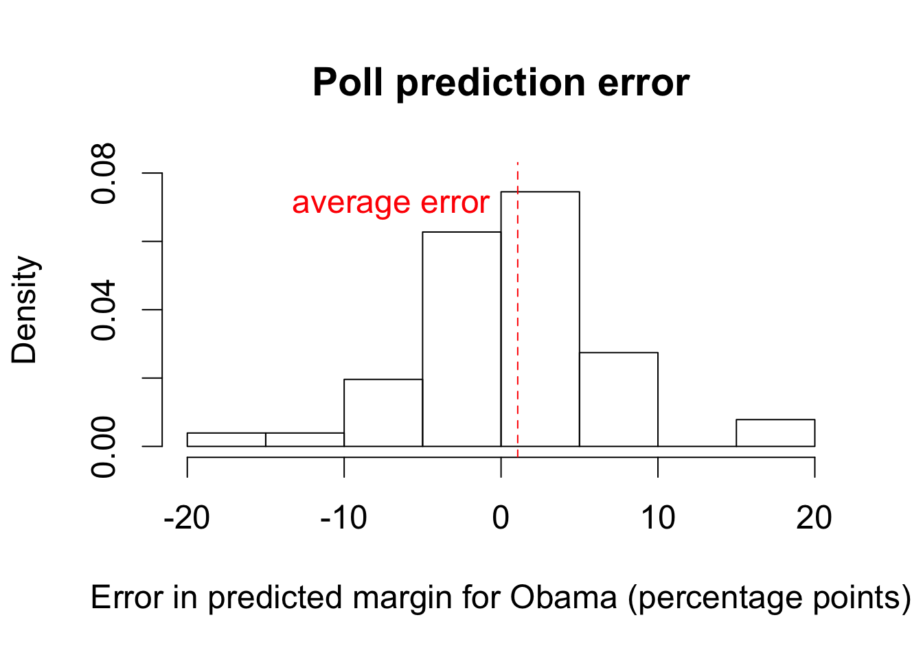
errors <- pres08$margin - poll.pred
names(errors) <- st.names # add state names
mean(errors) # mean prediction error
## [1] 1.062092
sqrt(mean(errors^2))
## [1] 5.90894
par(cex = 1.5)
## histogram
hist(errors, freq = FALSE, ylim = c(0, 0.08),
     main = "Poll prediction error",
     xlab = "Error in predicted margin for Obama (percentage points)")
## add mean
abline(v = mean(errors), lty = "dashed", col = "red")
text(x = -7, y = 0.07, "average error", col = "red")
par(cex = 1.5)
## type = "n" generates "empty" plot
plot(poll.pred, pres08$margin, type = "n", main = "", xlab = "Poll results",
     xlim = c(-40, 90), ylim = c(-40, 90), ylab = "Actual election results")
## add state abbreviations
text(x = poll.pred, y = pres08$margin, labels = pres08$state, col = "blue")
## lines
abline(a = 0, b = 1, lty = "dashed") # 45 degree line
abline(v = 0)  # vertical line at 0
abline(h = 0)  # horizontal line at 0
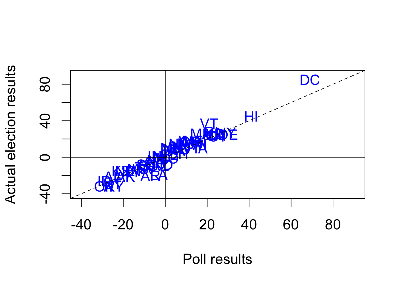
## which state polls called wrong?
pres08$state[sign(poll.pred) != sign(pres08$margin)]
## [1] "IN" "MO" "NC"
## what was the actual margin for these states?
pres08$margin[sign(poll.pred) != sign(pres08$margin)]
## [1] 1 -1 1
## actual results: total number of electoral votes won by Obama
sum(pres08$EV[pres08$margin > 0])
## [1] 364
## poll prediction
sum(pres08$EV[poll.pred > 0])
## [1] 349
## load the data
data("pollsUS08", package = "qss")
## compute number of days to the election as before
pollsUS08$middate <- as.Date(pollsUS08$middate)
pollsUS08$DaysToElection <- as.Date("2008-11-04") - pollsUS08$middate
## empty vectors to store predictions
Obama.pred <- McCain.pred <- rep(NA, 90)
for (i in 1:90) {
## take all polls conducted within the past 7 days
week.data <- subset(pollsUS08, subset = ((DaysToElection <= (90 - i + 7))
& (DaysToElection > (90 - i))))
## compute support for each candidate using the average
Obama.pred[i] <- mean(week.data$Obama)
McCain.pred[i] <- mean(week.data$McCain)
}
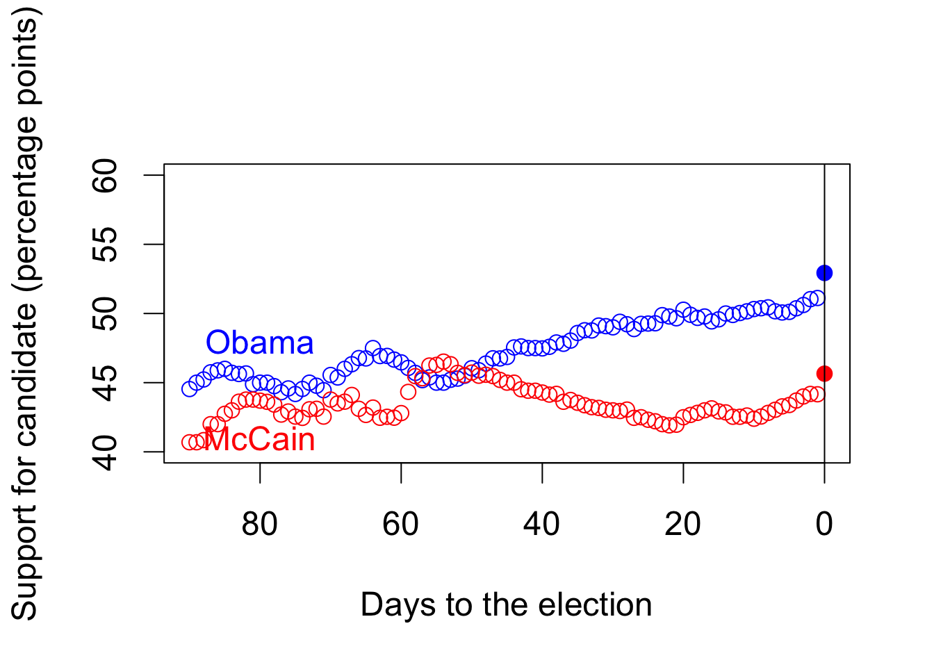
par(cex = 1.5)
## plot going from 90 days to 1 day before the election
plot(90:1, Obama.pred, type = "b", xlim = c(90, 0), ylim = c(40, 60),
col = "blue", xlab = "Days to the election",
ylab = "Support for candidate (percentage points)")
## `type = "b"' gives plot that includes both points and lines
lines(90:1, McCain.pred, type = "b", col = "red")
## actual election results: pch = 19 gives solid circles
points(0, 52.93, pch = 19, col = "blue")
points(0, 45.65, pch = 19, col = "red")
## line indicating the election day
abline(v = 0)
## labeling candidates
text(80, 48, "Obama", col = "blue")
text(80, 41, "McCain", col = "red")
Section 4.2: Linear Regression
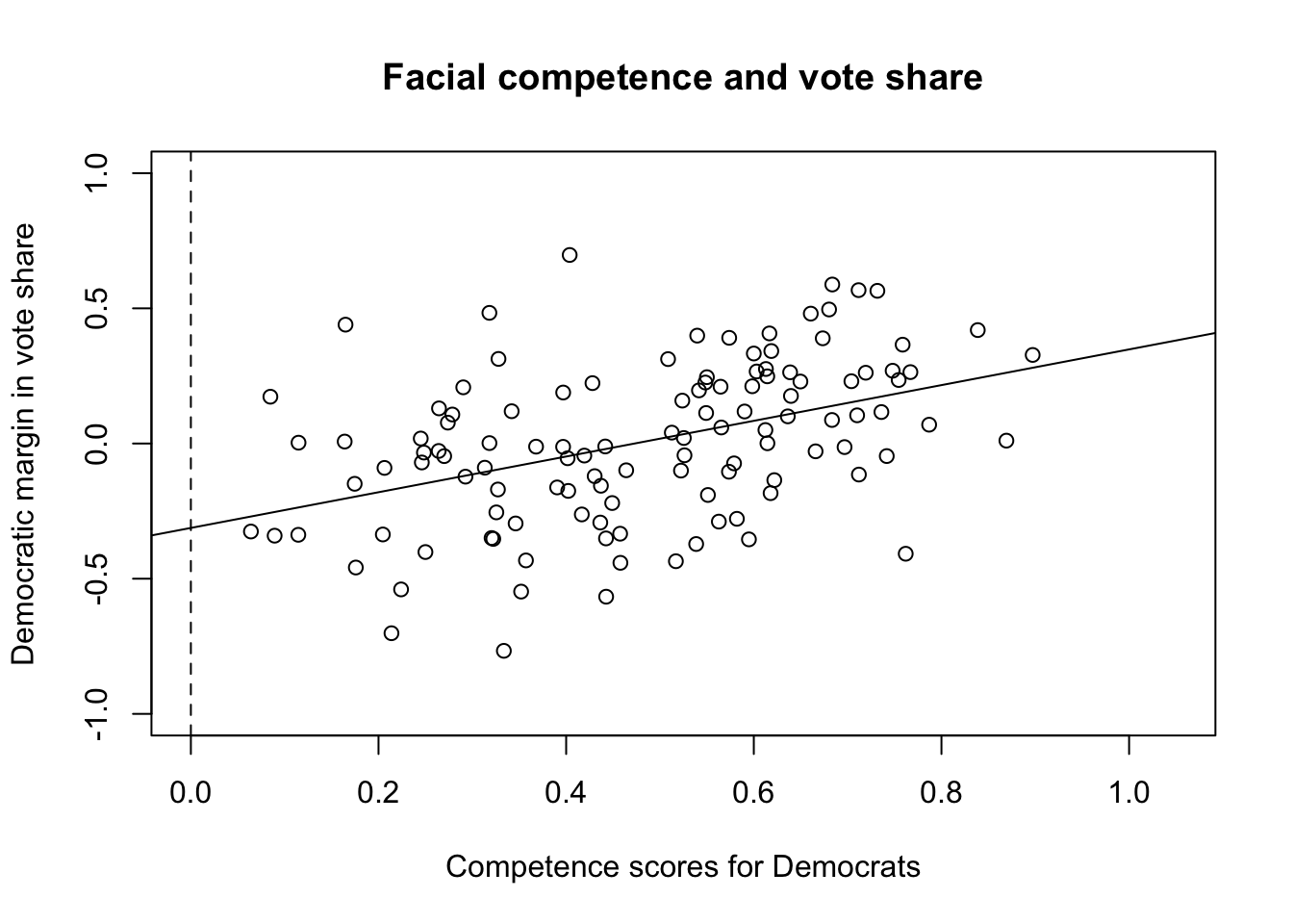
Section 4.2.1: Facial Appearance and Election Outcomes
## load the data
data("face", package = "qss")
## two-party vote share for Democrats and Republicans
face$d.share <- face$d.votes / (face$d.votes + face$r.votes)
face$r.share <- face$r.votes / (face$d.votes + face$r.votes)
face$diff.share <- face$d.share - face$r.share

par(cex = 1.5)
plot(face$d.comp, face$diff.share, pch = 16,
     col = ifelse(face$w.party == "R", "red", "blue"),
     xlim = c(0, 1), ylim = c(-1, 1),
     xlab = "Competence scores for Democrats",
     ylab = "Democratic margin in vote share",
     main = "Facial competence and vote share")
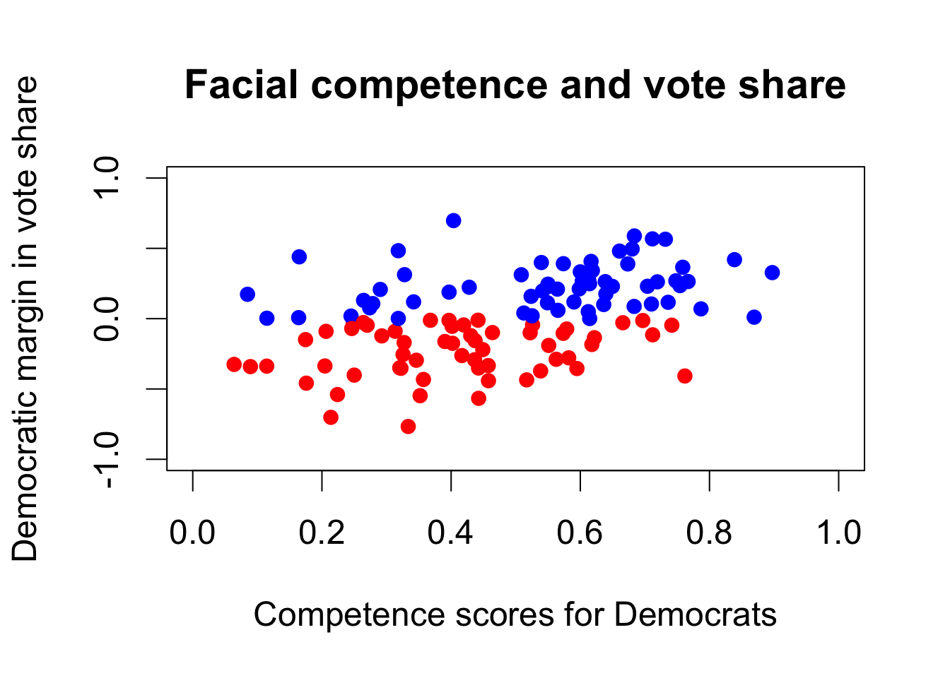
Section 4.2.2: Correlation and Scatter Plots
cor(face$d.comp, face$diff.share)
## [1] 0.4327743
Section 4.2.3: Least Squares
fit <- lm(diff.share ~ d.comp, data = face) # fit the model
fit
##
## Call:
## lm(formula = diff.share ~ d.comp, data = face)
##
## Coefficients:
## (Intercept)       d.comp
##     -0.3122       0.6604
## lm(face$diff.share ~ face$d.comp)
coef(fit)  # get estimated coefficients
## (Intercept)      d.comp
##  -0.3122259   0.6603815
head(fitted(fit)) # get fitted or predicted values
##           1           2           3           4           5           6
##  0.06060411 -0.08643340  0.09217061  0.04539236  0.13698690 -0.10057206
plot(face$d.comp, face$diff.share, xlim = c(0, 1.05), ylim = c(-1,1),
     xlab = "Competence scores for Democrats",
     ylab = "Democratic margin in vote share",
     main = "Facial competence and vote share")
abline(fit) # add regression line
abline(v = 0, lty = "dashed")
epsilon.hat <- resid(fit)  # residuals
sqrt(mean(epsilon.hat^2))  # RMSE
## [1] 0.2642361
Section 4.2.4: Regression Towards the Mean
Section 4.2.5: Merging Data Sets in R
data("pres12", package = "qss")  # load 2012 data
## quick look at two data sets
head(pres08)
##   state.name state Obama McCain EV margin
## 1    Alabama    AL    39     60  9    -21
## 2     Alaska    AK    38     59  3    -21
## 3    Arizona    AZ    45     54 10     -9
## 4   Arkansas    AR    39     59  6    -20
## 5 California    CA    61     37 55     24
## 6   Colorado    CO    54     45  9      9
head(pres12)
##   state Obama Romney EV
## 1    AL    38     61  9
## 2    AK    41     55  3
## 3    AZ    45     54 11
## 4    AR    37     61  6
## 5    CA    60     37 55
## 6    CO    51     46  9
## merge two data frames
pres <- merge(pres08, pres12, by = "state")

## summarize the merged data frame
summary(pres)
##     state            state.name           Obama.x          McCain
##  Length:51          Length:51          Min.   :33.00   Min.   : 7.00
##  Class :character   Class :character   1st Qu.:43.00   1st Qu.:40.00
##  Mode  :character   Mode  :character   Median :51.00   Median :47.00
##                                        Mean   :51.37   Mean   :47.06
##                                        3rd Qu.:57.50   3rd Qu.:56.00
##                                        Max.   :92.00   Max.   :66.00
##       EV.x           margin           Obama.y          Romney
##  Min.   : 3.00   Min.   :-32.000   Min.   :25.00   Min.   : 7.00
##  1st Qu.: 4.50   1st Qu.:-13.000   1st Qu.:40.50   1st Qu.:41.00
##  Median : 8.00   Median :  4.000   Median :51.00   Median :48.00
##  Mean   :10.55   Mean   :  4.314   Mean   :49.06   Mean   :49.04
##  3rd Qu.:11.50   3rd Qu.: 17.500   3rd Qu.:56.00   3rd Qu.:58.00
##  Max.   :55.00   Max.   : 85.000   Max.   :91.00   Max.   :73.00
##       EV.y
##  Min.   : 3.00
##  1st Qu.: 4.50
##  Median : 8.00
##  Mean   :10.55
##  3rd Qu.:11.50
##  Max.   :55.00
## change the variable name for illustration
names(pres12)[1] <- "state.abb"

## merging data sets using the variables of different names
pres <- merge(pres08, pres12, by.x = "state", by.y = "state.abb")
summary(pres)
##     state            state.name           Obama.x          McCain
##  Length:51          Length:51          Min.   :33.00   Min.   : 7.00
##  Class :character   Class :character   1st Qu.:43.00   1st Qu.:40.00
##  Mode  :character   Mode  :character   Median :51.00   Median :47.00
##                                        Mean   :51.37   Mean   :47.06
##                                        3rd Qu.:57.50   3rd Qu.:56.00
##                                        Max.   :92.00   Max.   :66.00
##       EV.x           margin           Obama.y          Romney
##  Min.   : 3.00   Min.   :-32.000   Min.   :25.00   Min.   : 7.00
##  1st Qu.: 4.50   1st Qu.:-13.000   1st Qu.:40.50   1st Qu.:41.00
##  Median : 8.00   Median :  4.000   Median :51.00   Median :48.00
##  Mean   :10.55   Mean   :  4.314   Mean   :49.06   Mean   :49.04
##  3rd Qu.:11.50   3rd Qu.: 17.500   3rd Qu.:56.00   3rd Qu.:58.00
##  Max.   :55.00   Max.   : 85.000   Max.   :91.00   Max.   :73.00
##       EV.y
##  Min.   : 3.00
##  1st Qu.: 4.50
##  Median : 8.00
##  Mean   :10.55
##  3rd Qu.:11.50
##  Max.   :55.00
## cbinding two data frames
pres1 <- cbind(pres08, pres12)
## this shows all variables are kept
summary(pres1)
##   state.name           state               Obama           McCain
##  Length:51          Length:51          Min.   :33.00   Min.   : 7.00
##  Class :character   Class :character   1st Qu.:43.00   1st Qu.:40.00
##  Mode  :character   Mode  :character   Median :51.00   Median :47.00
##                                        Mean   :51.37   Mean   :47.06
##                                        3rd Qu.:57.50   3rd Qu.:56.00
##                                        Max.   :92.00   Max.   :66.00
##        EV            margin         state.abb             Obama
##  Min.   : 3.00   Min.   :-32.000   Length:51          Min.   :25.00
##  1st Qu.: 4.50   1st Qu.:-13.000   Class :character   1st Qu.:40.50
##  Median : 8.00   Median :  4.000   Mode  :character   Median :51.00
##  Mean   :10.55   Mean   :  4.314                      Mean   :49.06
##  3rd Qu.:11.50   3rd Qu.: 17.500                      3rd Qu.:56.00
##  Max.   :55.00   Max.   : 85.000                      Max.   :91.00
##      Romney            EV
##  Min.   : 7.00   Min.   : 3.00
##  1st Qu.:41.00   1st Qu.: 4.50
##  Median :48.00   Median : 8.00
##  Mean   :49.04   Mean   :10.55
##  3rd Qu.:58.00   3rd Qu.:11.50
##  Max.   :73.00   Max.   :55.00
## DC and DE are flipped in this alternative approach
pres1[8:9, ]
##   state.name state Obama McCain EV margin state.abb Obama Romney EV
## 8       D.C.    DC    92      7  3     85        DE    59     40  3
## 9   Delaware    DE    62     37  3     25        DC    91      7  3
## merge() does not have this problem
pres[8:9, ]
##   state state.name Obama.x McCain EV.x margin Obama.y Romney EV.y
## 8    DC       D.C.      92      7    3     85      91      7    3
## 9    DE   Delaware      62     37    3     25      59     40    3
pres$Obama2008.z <- scale(pres$Obama.x)
pres$Obama2012.z <- scale(pres$Obama.y)

## intercept is estimated essentially zero
fit1 <- lm(Obama2012.z ~ Obama2008.z, data = pres)
fit1
##
## Call:
## lm(formula = Obama2012.z ~ Obama2008.z, data = pres)
##
## Coefficients:
## (Intercept)  Obama2008.z
##  -3.521e-17    9.834e-01
## regression without an intercept; estimated slope is identical
fit1 <- lm(Obama2012.z ~ -1 + Obama2008.z, data = pres)
fit1
##
## Call:
## lm(formula = Obama2012.z ~ -1 + Obama2008.z, data = pres)
##
## Coefficients:
## Obama2008.z
##      0.9834
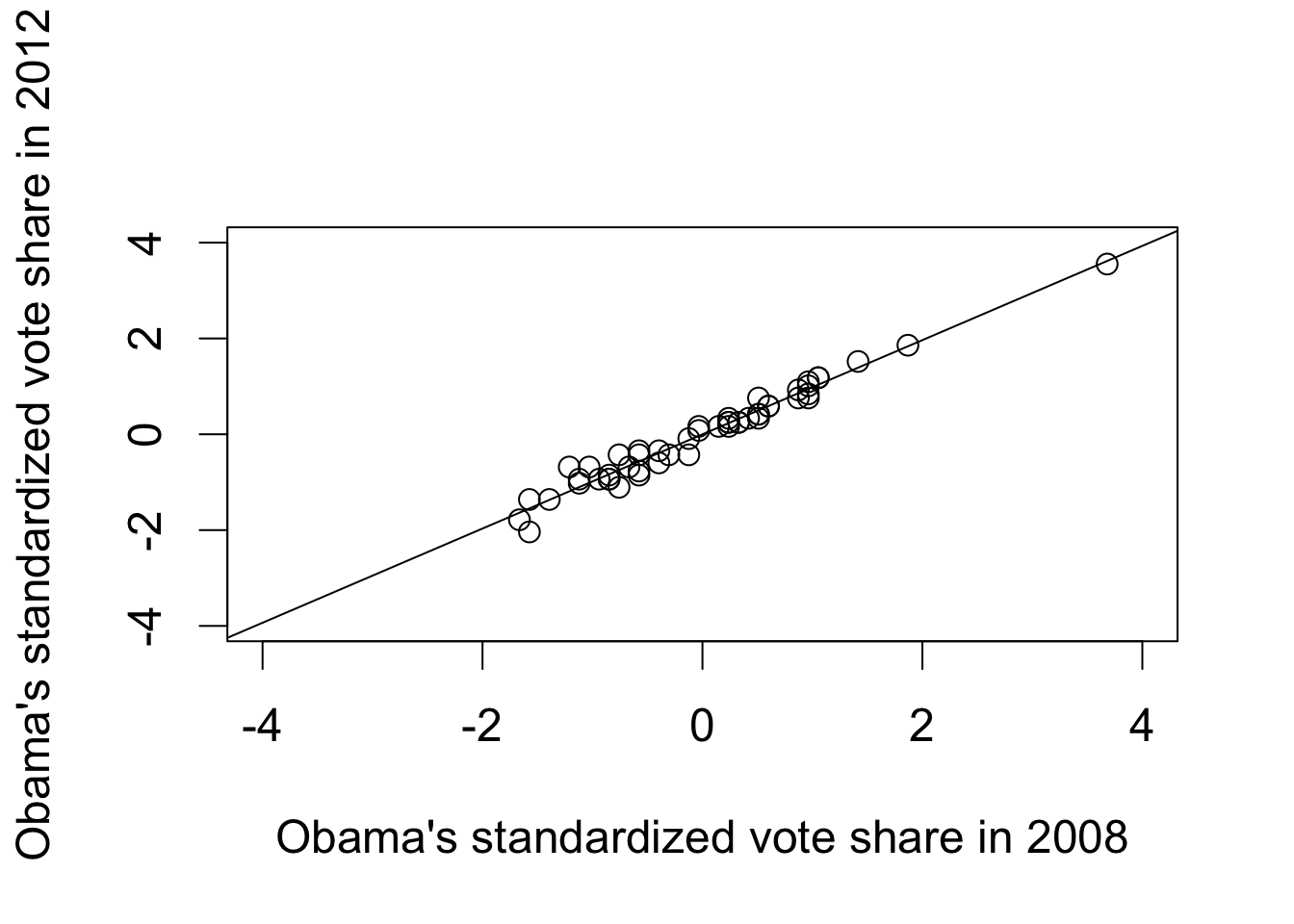
par(cex = 1.5)
plot(pres$Obama2008.z, pres$Obama2012.z, xlim = c(-4, 4), ylim = c(-4, 4),
     xlab = "Obama's standardized vote share in 2008",
     ylab = "Obama's standardized vote share in 2012")
abline(fit1) # draw a regression line
## bottom quartile
mean((pres$Obama2012.z >
          pres$Obama2008.z)[pres$Obama2008.z
                            <= quantile(pres$Obama2008.z, 0.25)])
## [1] 0.5714286
## top quartile
mean((pres$Obama2012.z >
          pres$Obama2008.z)[pres$Obama2008.z
                            >= quantile(pres$Obama2008.z, 0.75)])
## [1] 0.4615385
Section 4.2.6: Model Fit
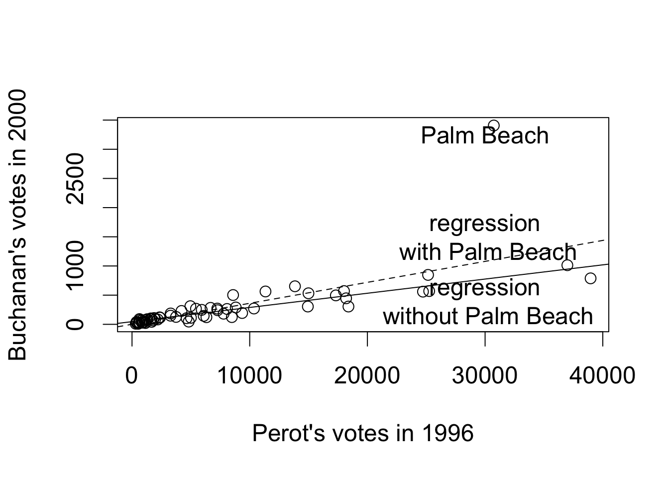
data("florida", package = "qss")

## regress Buchanan's 2000 votes on Perot's 1996 votes
fit2 <- lm(Buchanan00 ~ Perot96, data = florida)
fit2
##
## Call:
## lm(formula = Buchanan00 ~ Perot96, data = florida)
##
## Coefficients:
## (Intercept)      Perot96
##     1.34575      0.03592
## compute TSS (total sum of squares) and SSR (sum of squared residuals)
TSS2 <- sum((florida$Buchanan00 - mean(florida$Buchanan00))^2)
SSR2 <- sum(resid(fit2)^2)

## Coefficient of determination
(TSS2 - SSR2) / TSS2
## [1] 0.5130333
R2 <- function(fit) {
    resid <- resid(fit) # residuals
    y <- fitted(fit) + resid # outcome variable
    TSS <- sum((y - mean(y))^2)
    SSR <- sum(resid^2)
    R2 <- (TSS - SSR) / TSS
    return(R2)
}
R2(fit2)
## [1] 0.5130333
## built-in R function
summary(fit2)$r.squared
## [1] 0.5130333
R2(fit1)
## [1] 0.9671579
par(cex = 1.5)
plot(fitted(fit2), resid(fit2), xlim = c(0, 1500), ylim = c(-750, 2500),
     xlab = "Fitted values", ylab = "Residuals")
abline(h = 0)
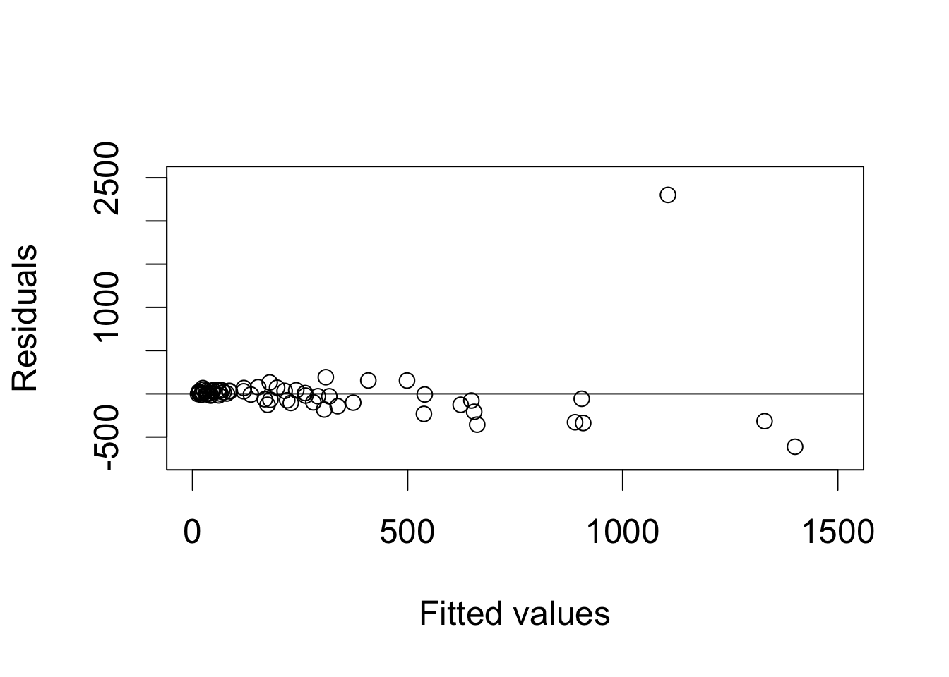
florida$county[resid(fit2) == max(resid(fit2))]
## [1] "PalmBeach"
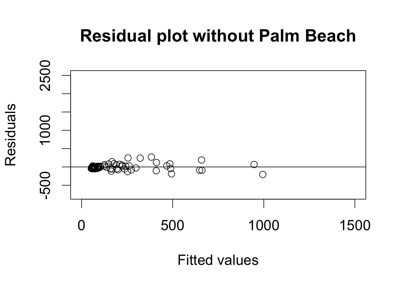
## data without Palm Beach
florida.pb <- subset(florida, subset = (county != "PalmBeach"))

fit3 <- lm(Buchanan00 ~ Perot96, data = florida.pb)
fit3
##
## Call:
## lm(formula = Buchanan00 ~ Perot96, data = florida.pb)
##
## Coefficients:
## (Intercept)      Perot96
##    45.84193      0.02435
## R^2 or coefficient of determination
R2(fit3)
## [1] 0.8511675
par(cex = 1.5)
## residual plot
plot(fitted(fit3), resid(fit3), xlim = c(0, 1500), ylim = c(-750, 2500),
     xlab = "Fitted values", ylab = "Residuals",
     main = "Residual plot without Palm Beach")
abline(h = 0) # horizontal line at 0
plot(florida$Perot96, florida$Buchanan00, xlab = "Perot's votes in 1996",
     ylab = "Buchanan's votes in 2000")
abline(fit2, lty = "dashed") # regression with Palm Beach
abline(fit3) # regression without Palm Beach
text(30000, 3250, "Palm Beach")
text(30000, 1500, "regression\n with Palm Beach")
text(30000, 400, "regression\n without Palm Beach")
Section 4.3: Regression and Causation
Section 4.3.1: Randomized Experiments
data("women", package = "qss")

## proportion of female politicians in reserved GP vs. unreserved GP
mean(women$female[women$reserved == 1])
## [1] 1
mean(women$female[women$reserved == 0])
## [1] 0.07476636
## drinking-water facilities
mean(women$water[women$reserved == 1]) -
    mean(women$water[women$reserved == 0])
## [1] 9.252423
## irrigation facilities
mean(women$irrigation[women$reserved == 1]) -
    mean(women$irrigation[women$reserved == 0])
## [1] -0.3693319
lm(water ~ reserved, data = women)
##
## Call:
## lm(formula = water ~ reserved, data = women)
##
## Coefficients:
## (Intercept)     reserved
##      14.738        9.252
lm(irrigation ~ reserved, data = women)
##
## Call:
## lm(formula = irrigation ~ reserved, data = women)
##
## Coefficients:
## (Intercept)     reserved
##      3.3879      -0.3693
Section 4.3.2: Regression with Multiple Predictors
data("social", package = "qss")
levels(social$messages) # base level is `Civic'
## NULL
fit <- lm(primary2006 ~ messages, data = social)
fit
##
## Call:
## lm(formula = primary2006 ~ messages, data = social)
##
## Coefficients:
##       (Intercept)    messagesControl  messagesHawthorne
##          0.314538          -0.017899           0.007837
## messagesNeighbors
##          0.063411
## ## create indicator variables
## social$Control <- ifelse(social$messages == "Control", 1, 0)
## social$Hawthorne <- ifelse(social$messages == "Hawthorne", 1, 0)
## social$Neighbors <- ifelse(social$messages == "Neighbors", 1, 0)
## ## fit the same regression as above by directly using indicator variables
## lm(primary2006 ~ Control + Hawthorne + Neighbors, data = social)

## create a data frame with unique values of `messages'
unique.messages <- data.frame(messages = unique(social$messages))
unique.messages
##     messages
## 1 Civic Duty
## 2  Hawthorne
## 3    Control
## 4  Neighbors
## make prediction for each observation from this new data frame
predict(fit, newdata = unique.messages)
##         1         2         3         4
## 0.3145377 0.3223746 0.2966383 0.3779482
## sample average
tapply(social$primary2006, social$messages, mean)
## Civic Duty    Control  Hawthorne  Neighbors
##  0.3145377  0.2966383  0.3223746  0.3779482
## linear regression without intercept
fit.noint <- lm(primary2006 ~ -1 + messages, data = social)
fit.noint
##
## Call:
## lm(formula = primary2006 ~ -1 + messages, data = social)
##
## Coefficients:
## messagesCivic Duty     messagesControl   messagesHawthorne
##             0.3145              0.2966              0.3224
##  messagesNeighbors
##             0.3779
## estimated average effect of `Neighbors' condition
coef(fit)["messagesNeighbors"] - coef(fit)["messagesControl"]
## messagesNeighbors
##        0.08130991
## difference in means
mean(social$primary2006[social$messages == "Neighbors"]) -
    mean(social$primary2006[social$messages == "Control"])
## [1] 0.08130991
## adjusted Rsquare
adjR2 <- function(fit) {
    resid <- resid(fit) # residuals
    y <- fitted(fit) + resid # outcome
    n <- length(y)
    TSS.adj <- sum((y - mean(y))^2) / (n - 1)
    SSR.adj <- sum(resid^2) / (n - length(coef(fit)))
    R2.adj <- 1 - SSR.adj / TSS.adj
    return(R2.adj)
}
adjR2(fit)
## [1] 0.003272788
R2(fit) # unadjusted Rsquare calculation
## [1] 0.003282564
summary(fit)$adj.r.squared
## [1] 0.003272788
Section 4.3.3: Heterogenous Treatment Effects
## average treatment effect (ate) among those who voted in 2004 primary
social.voter <- subset(social, primary2004 == 1)

ate.voter <-
    mean(social.voter$primary2006[social.voter$messages == "Neighbors"]) -
        mean(social.voter$primary2006[social.voter$messages == "Control"])
ate.voter
## [1] 0.09652525
## average effect among those who did not vote
social.nonvoter <- subset(social, primary2004 == 0)

ate.nonvoter <-
    mean(social.nonvoter$primary2006[social.nonvoter$messages == "Neighbors"]) -
        mean(social.nonvoter$primary2006[social.nonvoter$messages == "Control"])
ate.nonvoter
## [1] 0.06929617
## difference
ate.voter - ate.nonvoter
## [1] 0.02722908
## subset neighbors and control groups
social.neighbor <- subset(social, (messages == "Control") |
                              (messages == "Neighbors"))

## standard way to generate main and interaction effects
fit.int <- lm(primary2006 ~ primary2004 + messages + primary2004:messages,
              data = social.neighbor)
fit.int
##
## Call:
## lm(formula = primary2006 ~ primary2004 + messages + primary2004:messages,
##     data = social.neighbor)
##
## Coefficients:
##                   (Intercept)                    primary2004
##                       0.23711                        0.14870
##             messagesNeighbors  primary2004:messagesNeighbors
##                       0.06930                        0.02723
## lm(primary2006 ~ primary2004 * messages, data = social.neighbor)

social.neighbor$age <- 2008 - social.neighbor$yearofbirth
summary(social.neighbor$age)
##    Min. 1st Qu.  Median    Mean 3rd Qu.    Max.
##   22.00   43.00   52.00   51.82   61.00  108.00
fit.age <- lm(primary2006 ~ age * messages, data = social.neighbor)
fit.age
##
## Call:
## lm(formula = primary2006 ~ age * messages, data = social.neighbor)
##
## Coefficients:
##           (Intercept)                    age      messagesNeighbors
##             0.0894768              0.0039982              0.0485728
## age:messagesNeighbors
##             0.0006283
## age = 25, 45, 65, 85 in Neighbors group
age.neighbor <- data.frame(age = seq(from = 25, to = 85, by = 20),
                           messages = "Neighbors")

## age = 25, 45, 65, 85 in Control group
age.control <- data.frame(age = seq(from = 25, to = 85, by = 20),
                          messages = "Control")

## average treatment effect for age = 25, 45, 65, 85
ate.age <- predict(fit.age, newdata = age.neighbor) -
    predict(fit.age, newdata = age.control)

ate.age
##          1          2          3          4
## 0.06428051 0.07684667 0.08941283 0.10197899
fit.age2 <- lm(primary2006 ~ age + I(age^2) + messages + age:messages +
                 I(age^2):messages, data = social.neighbor)

fit.age2
##
## Call:
## lm(formula = primary2006 ~ age + I(age^2) + messages + age:messages +
##     I(age^2):messages, data = social.neighbor)
##
## Coefficients:
##                (Intercept)                         age
##                 -9.700e-02                   1.172e-02
##                   I(age^2)           messagesNeighbors
##                 -7.389e-05                  -5.275e-02
##      age:messagesNeighbors  I(age^2):messagesNeighbors
##                  4.804e-03                  -3.961e-05
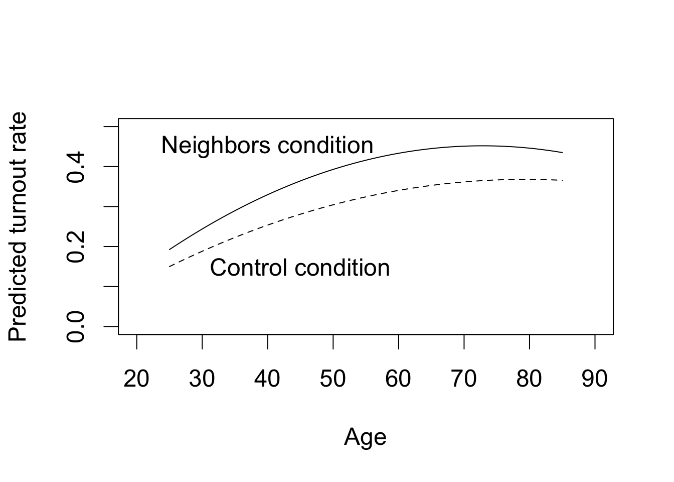
## predicted turnout rate under the ``Neighbors'' treatment condition
yT.hat <- predict(fit.age2,
                  newdata = data.frame(age = 25:85, messages = "Neighbors"))

## predicted turnout rate under the control condition
yC.hat <- predict(fit.age2,
                  newdata = data.frame(age = 25:85, messages = "Control"))

par(cex = 1.5)
## plotting the predicted turnout rate under each condition
plot(x = 25:85, y = yT.hat, type = "l", xlim = c(20, 90), ylim = c(0, 0.5),
     xlab = "Age", ylab = "Predicted turnout rate")
lines(x = 25:85, y = yC.hat, lty = "dashed")
text(40, 0.45, "Neighbors condition")
text(45, 0.15, "Control condition")
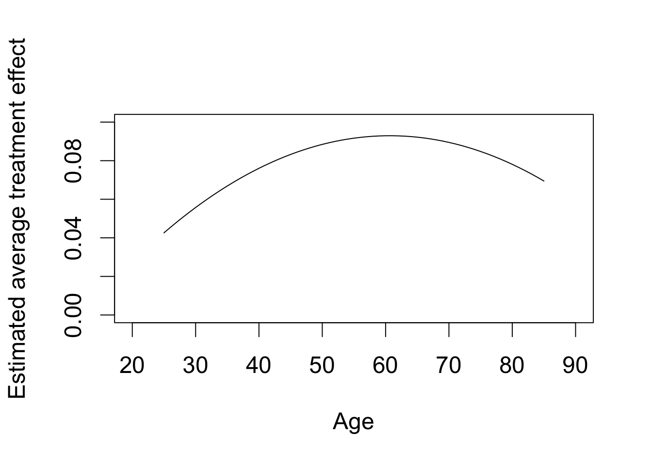
## plotting the average treatment effect as a function of age
plot(x = 25:85, y = yT.hat - yC.hat, type = "l", xlim = c(20, 90),
     ylim = c(0, 0.1), xlab = "Age",
     ylab = "Estimated average treatment effect")
Section 4.3.4: Regression Discontinuity Design
## load the data and subset them into two parties
data("MPs", package = "qss")
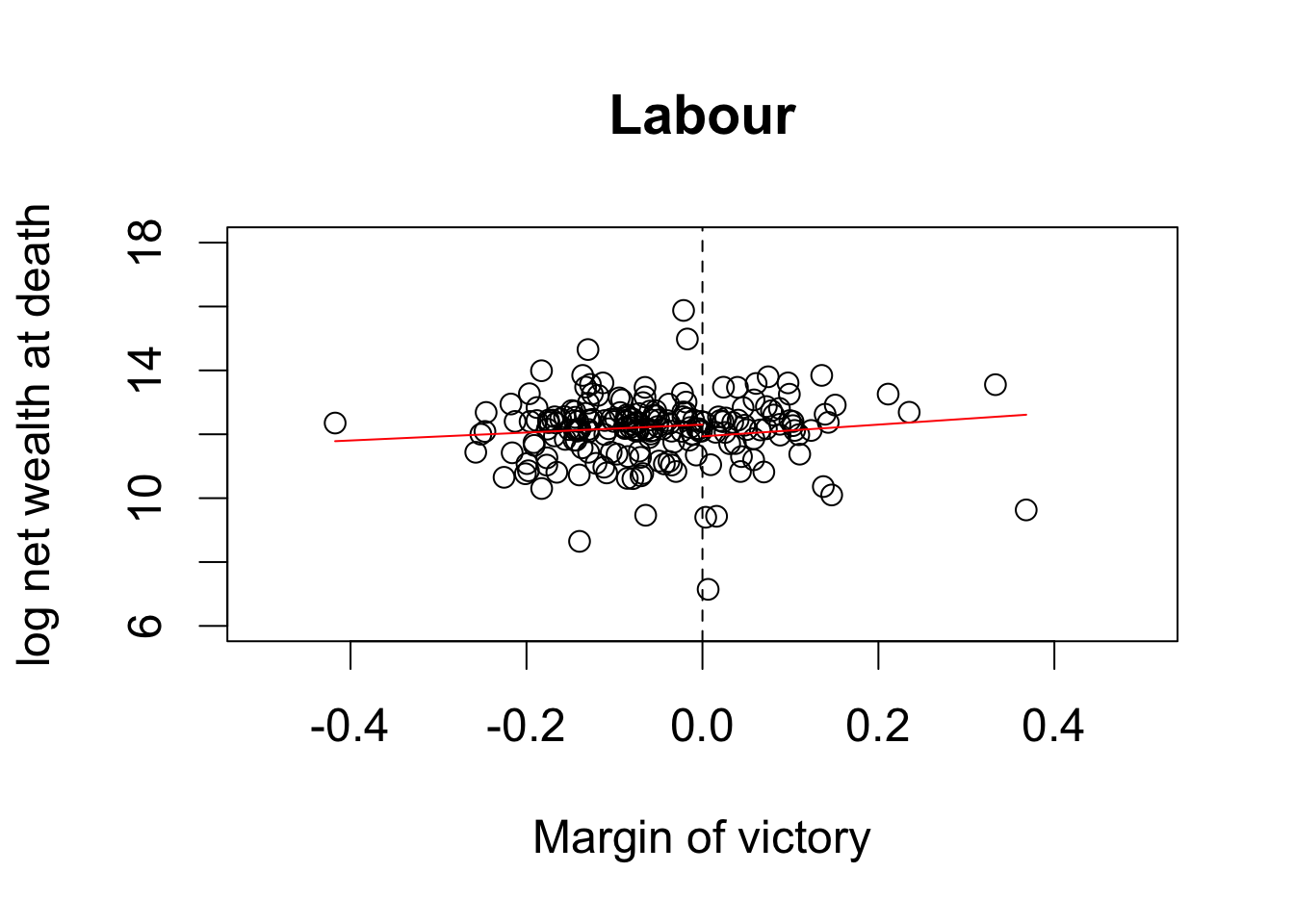
MPs.labour <- subset(MPs, subset = (party == "labour"))
MPs.tory <- subset(MPs, subset = (party == "tory"))
## two regressions for Labour: negative and positive margin
labour.fit1 <- lm(ln.net ~ margin,
data = MPs.labour[MPs.labour$margin < 0, ])
labour.fit2 <- lm(ln.net ~ margin,
data = MPs.labour[MPs.labour$margin > 0, ])
## two regressions for Tory: negative and positive margin
tory.fit1 <- lm(ln.net ~ margin, data = MPs.tory[MPs.tory$margin < 0, ])
tory.fit2 <- lm(ln.net ~ margin, data = MPs.tory[MPs.tory$margin > 0, ])
## Labour: range of predictions
y1l.range <- c(min(MPs.labour$margin), 0) # min to 0
y2l.range <- c(0, max(MPs.labour$margin)) # 0 to max
## prediction
y1.labour <- predict(labour.fit1, newdata = data.frame(margin = y1l.range))
y2.labour <- predict(labour.fit2, newdata = data.frame(margin = y2l.range))
## Tory: range of predictions
y1t.range <- c(min(MPs.tory$margin), 0) # min to 0
y2t.range <- c(0, max(MPs.tory$margin)) # 0 to max
## predict outcome
y1.tory <- predict(tory.fit1, newdata = data.frame(margin = y1t.range))
y2.tory <- predict(tory.fit2, newdata = data.frame(margin = y2t.range))
par(cex = 1.5)
## scatterplot with regression lines for labour
plot(MPs.labour$margin, MPs.labour$ln.net, main = "Labour",
xlim = c(-0.5, 0.5), ylim = c(6, 18), xlab = "Margin of victory",
ylab = "log net wealth at death")
abline(v = 0, lty = "dashed")
## add regression lines
lines(y1l.range, y1.labour, col = "red")
lines(y2l.range, y2.labour, col = "red")
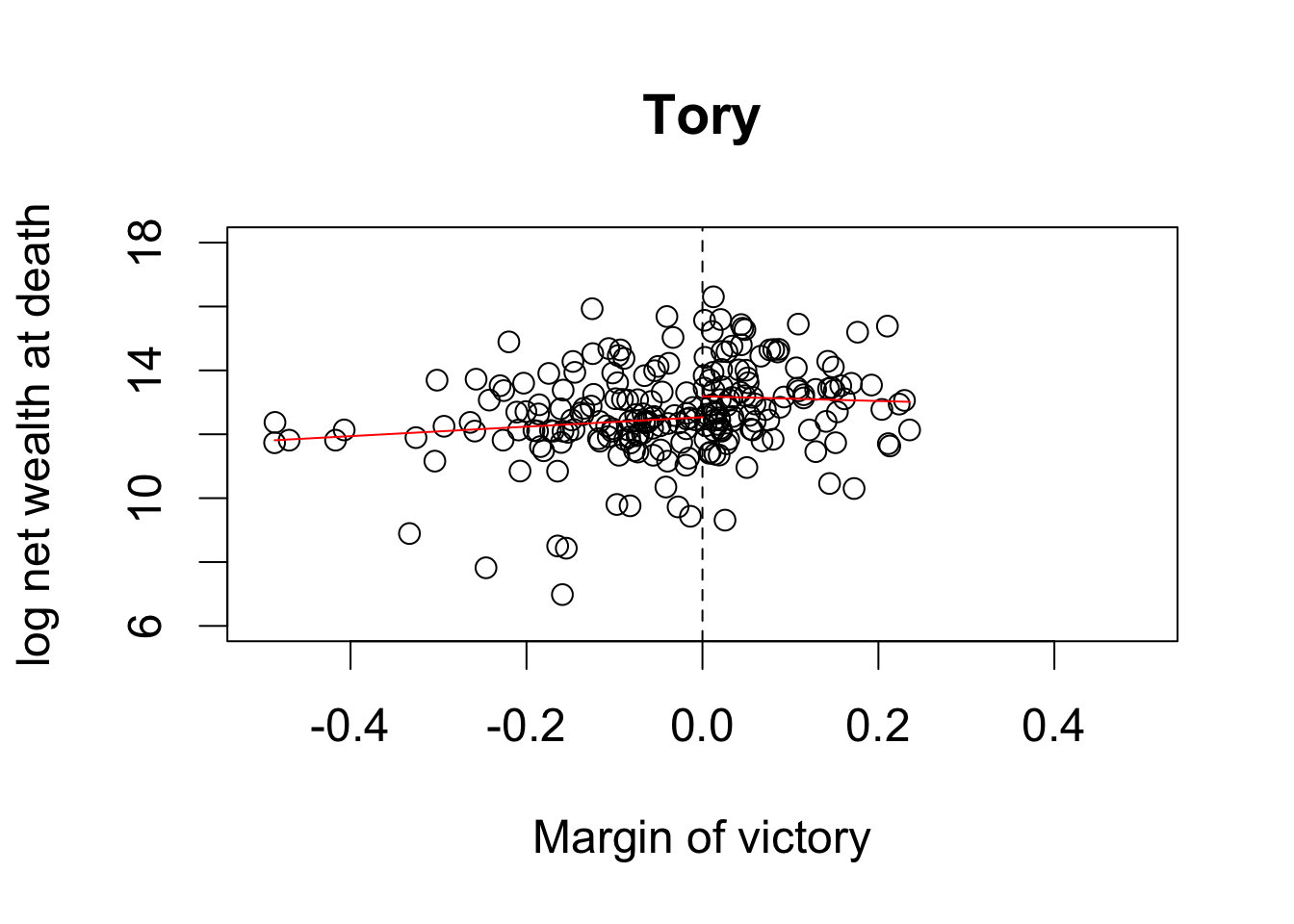
## scatterplot with regression lines for tory
plot(MPs.tory$margin, MPs.tory$ln.net, main = "Tory", xlim = c(-0.5, 0.5),
     ylim = c(6, 18), xlab = "Margin of victory",
     ylab = "log net wealth at death")
abline(v = 0, lty = "dashed")

## add regression lines
lines(y1t.range, y1.tory, col = "red")
lines(y2t.range, y2.tory, col = "red")
## average net wealth for Tory MP
tory.MP <- exp(y2.tory[1])
tory.MP
##        1
## 533813.5
## average net wealth for Tory non-MP
tory.nonMP <- exp(y1.tory[2])
tory.nonMP
##        2
## 278762.5
## causal effect in pounds
tory.MP - tory.nonMP
##        1
## 255050.9
## two regressions for Tory: negative and positive margin
tory.fit3 <- lm(margin.pre ~ margin, data = MPs.tory[MPs.tory$margin < 0, ])
tory.fit4 <- lm(margin.pre ~ margin, data = MPs.tory[MPs.tory$margin > 0, ])
## the difference between two intercepts is the estimated effect
coef(tory.fit4)[1] - coef(tory.fit3)[1]
## (Intercept)
## -0.01725578