Section 5.1: Textual Data
Section 5.1.1: The Disputed Authorship of ‘The Federalist Papers’
## load two required libraries
library(tm)
## Loading required package: NLP
library(SnowballC)

## load the raw corpus
corpus_dir <- system.file("extdata/federalist/", package = "qss")
corpus.raw <- Corpus(DirSource(corpus_dir, pattern = "\\.txt$"))
corpus.raw
## <<SimpleCorpus>>
## Metadata:  corpus specific: 1, document level (indexed): 0
## Content:  documents: 85
## make lower case
corpus.prep <- tm_map(corpus.raw, content_transformer(tolower))
## remove white space
corpus.prep <- tm_map(corpus.prep, stripWhitespace)
## remove punctuation
corpus.prep <- tm_map(corpus.prep, removePunctuation)

## remove numbers
corpus.prep <- tm_map(corpus.prep, removeNumbers)

head(stopwords("english"))
## [1] "i" "me" "my" "myself" "we" "our"
## remove stop words
corpus <- tm_map(corpus.prep, removeWords, stopwords("english"))

## finally stem remaining words
corpus <- tm_map(corpus, stemDocument)

## the output is truncated here to save space
content(corpus[[10]]) # Essay No. 10
## Warning in as.POSIXlt.POSIXct(Sys.time(), tz = "GMT"): unknown timezone
## 'zone/tz/2017c.1.0/zoneinfo/America/New_York'
## [1] "among numer advantag promis wellconstruct union none deserv accur develop tendenc break control violenc faction friend popular govern never find much alarm charact fate contempl propens danger vice will fail therefor set due valu plan without violat principl attach provid proper cure instabl injustic confus introduc public council truth mortal diseas popular govern everywher perish continu favorit fruit topic adversari liberti deriv specious declam valuabl improv made american constitut popular model ancient modern certain much admir unwarrant partial contend effectu obviat danger side wish expect complaint everywher heard consider virtuous citizen equal friend public privat faith public person liberti govern unstabl public good disregard conflict rival parti measur often decid accord rule justic right minor parti superior forc interest overbear major howev anxious may wish complaint foundat evid known fact will permit us deni degre true will found inde candid review situat distress labor erron charg oper govern will found time caus will alon account mani heaviest misfortun particular prevail increas distrust public engag alarm privat right echo one end contin must chiefli wholli effect unsteadi injustic factious spirit taint public administr faction understand number citizen whether amount major minor whole unit actuat common impuls passion interest advers right citizen perman aggreg interest communiti two method cure mischief faction one remov caus control effect two method remov caus faction one destroy liberti essenti exist give everi citizen opinion passion interest never truli said first remedi wors diseas liberti faction air fire aliment without instant expir less folli abolish liberti essenti polit life nourish faction wish annihil air essenti anim life impart fire destruct agenc second expedi impractic first unwis long reason man continu fallibl liberti exercis differ opinion will form long connect subsist reason selflov opinion passion will reciproc influenc former will object latter will attach divers faculti men right properti origin less insuper obstacl uniform interest protect faculti first object govern protect differ unequ faculti acquir properti possess differ degre kind properti immedi result influenc sentiment view respect proprietor ensu divis societi differ interest parti latent caus faction thus sown natur man see everywher brought differ degre activ accord differ circumst civil societi zeal differ opinion concern religion concern govern mani point well specul practic attach differ leader ambiti contend preemin power person descript whose fortun interest human passion turn divid mankind parti inflam mutual animos render much dispos vex oppress cooper common good strong propens mankind fall mutual animos substanti occas present frivol fanci distinct suffici kindl unfriend passion excit violent conflict common durabl sourc faction various unequ distribut properti hold without properti ever form distinct interest societi creditor debtor fall like discrimin land interest manufactur interest mercantil interest money interest mani lesser interest grow necess civil nation divid differ class actuat differ sentiment view regul various interf interest form princip task modern legisl involv spirit parti faction necessari ordinari oper govern man allow judg caus interest certain bias judgment improb corrupt integr equal nay greater reason bodi men unfit judg parti time yet mani import act legisl mani judici determin inde concern right singl person concern right larg bodi citizen differ class legisl advoc parti caus determin law propos concern privat debt question creditor parti one side debtor justic hold balanc yet parti must judg numer parti word power faction must expect prevail shall domest manufactur encourag degre restrict foreign manufactur question differ decid land manufactur class probabl neither sole regard justic public good apportion tax various descript properti act seem requir exact imparti yet perhap legisl act greater opportun temptat given predomin parti trampl rule justic everi shill overburden inferior number shill save pocket vain say enlighten statesmen will abl adjust clash interest render subservi public good enlighten statesmen will alway helm mani case can adjust made without take view indirect remot consider will rare prevail immedi interest one parti may find disregard right anoth good whole infer brought caus faction remov relief sought mean control effect faction consist less major relief suppli republican principl enabl major defeat sinist view regular vote may clog administr may convuls societi will unabl execut mask violenc form constitut major includ faction form popular govern hand enabl sacrific rule passion interest public good right citizen secur public good privat right danger faction time preserv spirit form popular govern great object inquiri direct let add great desideratum form govern can rescu opprobrium long labor recommend esteem adopt mankind mean object attain evid one two either exist passion interest major time must prevent major coexist passion interest must render number local situat unabl concert carri effect scheme oppress impuls opportun suffer coincid well know neither moral religi motiv can reli adequ control found injustic violenc individu lose efficaci proport number combin togeth proport efficaci becom need view subject may conclud pure democraci mean societi consist small number citizen assembl administ govern person can admit cure mischief faction common passion interest will almost everi case felt major whole communic concert result form govern noth check induc sacrific weaker parti obnoxi individu henc democraci ever spectacl turbul content ever found incompat person secur right properti general short live violent death theoret politician patron speci govern erron suppos reduc mankind perfect equal polit right time perfect equal assimil possess opinion passion republ mean govern scheme represent take place open differ prospect promis cure seek let us examin point vari pure democraci shall comprehend natur cure efficaci must deriv union two great point differ democraci republ first deleg govern latter small number citizen elect rest second greater number citizen greater sphere countri latter may extend effect first differ one hand refin enlarg public view pass medium chosen bodi citizen whose wisdom may best discern true interest countri whose patriot love justic will least like sacrific temporari partial consider regul may well happen public voic pronounc repres peopl will conson public good pronounc peopl conven purpos hand effect may invert men factious temper local prejudic sinist design may intrigu corrupt mean first obtain suffrag betray interest peopl question result whether small extens republ favor elect proper guardian public weal clear decid favor latter two obvious consider first place remark howev small republ may repres must rais certain number order guard cabal howev larg may must limit certain number order guard confus multitud henc number repres two case proport two constitu proport greater small republ follow proport fit charact less larg small republ former will present greater option consequ greater probabl fit choic next place repres will chosen greater number citizen larg small republ will difficult unworthi candid practic success vicious art elect often carri suffrag peopl free will like centr men possess attract merit diffus establish charact must confess case mean side inconveni will found lie enlarg much number elector render repres littl acquaint local circumst lesser interest reduc much render unduli attach littl fit comprehend pursu great nation object feder constitut form happi combin respect great aggreg interest refer nation local particular state legislatur point differ greater number citizen extent territori may brought within compass republican democrat govern circumst princip render factious combin less dread former latter smaller societi fewer probabl will distinct parti interest compos fewer distinct parti interest frequent will major found parti smaller number individu compos major smaller compass within place easili will concert execut plan oppress extend sphere take greater varieti parti interest make less probabl major whole will common motiv invad right citizen common motiv exist will difficult feel discov strength act unison besid impedi may remark conscious unjust dishonor purpos communic alway check distrust proport number whose concurr necessari henc clear appear advantag republ democraci control effect faction enjoy larg small republici enjoy union state compos advantag consist substitut repres whose enlighten view virtuous sentiment render superior local prejudic scheme injustic will deni represent union will like possess requisit endow consist greater secur afford greater varieti parti event one parti abl outnumb oppress rest equal degre increas varieti parti compris within union increas secur fine consist greater obstacl oppos concert accomplish secret wish unjust interest major extent union give palpabl advantag influenc factious leader may kindl flame within particular state will unabl spread general conflagr state religi sect may degener polit faction part confederaci varieti sect dispers entir face must secur nation council danger sourc rage paper money abolit debt equal divis properti improp wick project will less apt pervad whole bodi union particular member proport maladi like taint particular counti district entir state extent proper structur union therefor behold republican remedi diseas incid republican govern accord degre pleasur pride feel republican zeal cherish spirit support charact federalist"
Section 5.1.2: Document-Term Matrix
dtm <- DocumentTermMatrix(corpus)
dtm
## <<DocumentTermMatrix (documents: 85, terms: 4849)>>
## Non-/sparse entries: 44917/367248
## Sparsity           : 89%
## Maximal term length: 18
## Weighting          : term frequency (tf)
inspect(dtm[1:5, 1:8])
## <<DocumentTermMatrix (documents: 5, terms: 8)>>
## Non-/sparse entries: 18/22
## Sparsity           : 55%
## Maximal term length: 10
## Weighting          : term frequency (tf)
## Sample             :
##     Terms
## Docs abl absurd accid accord acknowledg act actuat add
##    1   1      1     1      1          1   1      1   1
##    2   0      0     0      0          0   0      0   0
##    3   2      0     0      1          2   1      1   1
##    4   1      0     0      1          0   1      0   0
##    5   0      0     0      0          0   1      0   0
dtm.mat <- as.matrix(dtm)
Section 5.1.3: Topic Discovery
library(wordcloud)
## Loading required package: RColorBrewer
wordcloud(colnames(dtm.mat), dtm.mat[12, ], max.words = 20) # essay No. 12

wordcloud(colnames(dtm.mat), dtm.mat[24, ], max.words = 20) # essay No. 24

stemCompletion(c("revenu", "commerc", "peac", "army"), corpus.prep)
##     revenu    commerc       peac       army
##  "revenue" "commerce"    "peace"     "army"
dtm.tfidf <- weightTfIdf(dtm) # tf-idf calculation

dtm.tfidf.mat <- as.matrix(dtm.tfidf)  # convert to matrix

## 10 most important words for Paper No. 12
head(sort(dtm.tfidf.mat[12, ], decreasing = TRUE), n = 10)
##     revenu contraband     patrol      excis      coast      trade
## 0.01905877 0.01886965 0.01886965 0.01876560 0.01592559 0.01473504
##        per        tax       cent     gallon
## 0.01420342 0.01295466 0.01257977 0.01257977
## 10 most important words for Paper No. 24
head(sort(dtm.tfidf.mat[24, ], decreasing = TRUE), n = 10)
##   garrison settlement   dockyard      spain       armi   frontier
## 0.02965511 0.01962294 0.01962294 0.01649040 0.01544256 0.01482756
##    arsenal    western       post     nearer
## 0.01308196 0.01306664 0.01236780 0.01166730
k <- 4  # number of clusters
## subset The Federalist papers written by Hamilton
hamilton <- c(1, 6:9, 11:13, 15:17, 21:36, 59:61, 65:85)
dtm.tfidf.hamilton <- dtm.tfidf.mat[hamilton, ]

## run k-means
km.out <- kmeans(dtm.tfidf.hamilton, centers = k)
km.out$iter # check the convergence; number of iterations may vary
## [1] 3
## label each centroid with the corresponding term
colnames(km.out$centers) <- colnames(dtm.tfidf.hamilton)

for (i in 1:k) { # loop for each cluster
    cat("CLUSTER", i, "\n")
    cat("Top 10 words:\n") # 10 most important terms at the centroid
    print(head(sort(km.out$centers[i, ], decreasing = TRUE), n = 10))
    cat("\n")
    cat("Federalist Papers classified: \n") # extract essays classified
    print(rownames(dtm.tfidf.hamilton)[km.out$cluster == i])
    cat("\n")
}
## CLUSTER 1
## Top 10 words:
##         tax       taxat      revenu       claus        land    merchant
## 0.011048535 0.010303867 0.008653646 0.008341649 0.006601163 0.005103442
##      export        upon         lay  manufactur
## 0.004999712 0.004907301 0.004799584 0.004781512
##
## Federalist Papers classified:
##  [1] "7"  "12" "21" "30" "31" "32" "33" "34" "35" "36"
##
## CLUSTER 2
## Top 10 words:
##       court       senat      presid        juri        upon       offic
## 0.008440690 0.005504293 0.004554328 0.004149586 0.003765824 0.003401184
##     impeach       nomin    governor   jurisdict
## 0.003313589 0.002831530 0.002752171 0.002684640
##
## Federalist Papers classified:
##  [1] "1"  "9"  "15" "16" "17" "22" "23" "27" "59" "60" "61" "65" "66" "68"
## [15] "69" "70" "71" "72" "73" "74" "75" "76" "77" "78" "79" "80" "81" "82"
## [29] "83" "84" "85"
##
## CLUSTER 3
## Top 10 words:
##     vacanc     recess      claus      senat    session       fill
## 0.06953047 0.04437713 0.04082617 0.03408008 0.03313305 0.03101140
##    appoint     presid      expir    unfound
## 0.02211662 0.01852025 0.01738262 0.01684465
##
## Federalist Papers classified:
## [1] "67"
##
## CLUSTER 4
## Top 10 words:
##        armi     militia    militari       navig   disciplin         war
## 0.011624485 0.011450433 0.008761049 0.005321748 0.004948897 0.004854514
##        peac    northern    frontier confederaci
## 0.004668017 0.004661314 0.004559462 0.004540867
##
## Federalist Papers classified:
## [1] "6"  "8"  "11" "13" "24" "25" "26" "28" "29"
Section 5.1.4: Authorship Prediction
## document-term matrix converted to matrix for manipulation
dtm1 <- as.matrix(DocumentTermMatrix(corpus.prep))
tfm <- dtm1 / rowSums(dtm1) * 1000 # term frequency per 1000 words

## words of interest
words <- c("although", "always", "commonly", "consequently",
           "considerable", "enough", "there", "upon", "while", "whilst")

## select only these words
tfm <- tfm[, words]

## essays written by Madison: `hamilton' defined earlier
madison <- c(10, 14, 37:48, 58)

## average among Hamilton/Madison essays
tfm.ave <- rbind(colSums(tfm[hamilton, ]) / length(hamilton),
                 colSums(tfm[madison, ]) / length(madison))
tfm.ave
##        although    always  commonly consequently considerable    enough
## [1,] 0.01756975 0.7527744 0.2630876   0.02600857    0.5435127 0.3955031
## [2,] 0.27058809 0.2006710 0.0000000   0.44878468    0.1601669 0.0000000
##         there      upon     while      whilst
## [1,] 4.417750 4.3986828 0.3700484 0.007055719
## [2,] 1.113252 0.2000269 0.0000000 0.380113114
author <- rep(NA, nrow(dtm1)) # a vector with missing values
author[hamilton] <- 1  # 1 if Hamilton
author[madison] <- -1  # -1 if Madison

## data frame for regression
author.data <- data.frame(author = author[c(hamilton, madison)],
                          tfm[c(hamilton, madison), ])

hm.fit <- lm(author ~ upon + there + consequently + whilst,
             data = author.data)
hm.fit
##
## Call:
## lm(formula = author ~ upon + there + consequently + whilst, data = author.data)
##
## Coefficients:
##  (Intercept)          upon         there  consequently        whilst
##     -0.26288       0.16678       0.09494      -0.44012      -0.65875
hm.fitted <- fitted(hm.fit) # fitted values
sd(hm.fitted)
## [1] 0.7180769
Section 5.1.5: Cross-Validation
## proportion of correctly classified essays by Hamilton
mean(hm.fitted[author.data$author == 1] > 0)
## [1] 1
## proportion of correctly classified essays by Madison
mean(hm.fitted[author.data$author == -1] < 0)
## [1] 1
n <- nrow(author.data)
hm.classify <- rep(NA, n) # a container vector with missing values

for (i in 1:n) {
    ## fit the model to the data after removing the ith observation
    sub.fit <- lm(author ~ upon + there + consequently + whilst,
                  data = author.data[-i, ]) # exclude ith row
    ## predict the authorship for the ith observation
    hm.classify[i] <- predict(sub.fit, newdata = author.data[i, ])
}

## proportion of correctly classified essays by Hamilton
mean(hm.classify[author.data$author == 1] > 0)
## [1] 1
## proportion of correctly classified essays by Madison
mean(hm.classify[author.data$author == -1] < 0)
## [1] 1
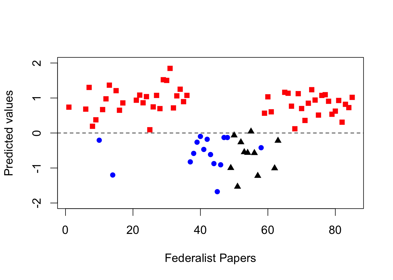
disputed <- c(49, 50:57, 62, 63) # 11 essays with disputed authorship
tf.disputed <- as.data.frame(tfm[disputed, ])

## prediction of disputed authorship
pred <- predict(hm.fit, newdata = tf.disputed)
pred # predicted values
##          49          50          51          52          53          54
## -0.99831799 -0.06759254 -1.53243206 -0.26288400 -0.54584900 -0.56566555
##          55          56          57          62          63
##  0.04376632 -0.57115610 -1.22289415 -1.00675456 -0.21939646
par(cex = 1.25)
## fitted values for essays authored by Hamilton; red squares
plot(hamilton, hm.fitted[author.data$author == 1], pch = 15,
     xlim = c(1, 85), ylim  = c(-2, 2), col = "red",
     xlab = "Federalist Papers", ylab = "Predicted values")
abline(h = 0, lty = "dashed")

## essays authored by Madison; blue circles
points(madison, hm.fitted[author.data$author == -1],
       pch = 16, col = "blue")

## disputed authorship; black triangles
points(disputed, pred, pch = 17)
Section 5.2: Network Data
Section 5.2.1: Marriage Network in Renaissance Florence
## the first column "FAMILY" of the CSV file represents row names
data("florentine", package = "qss")
florence <- data.frame(florentine, row.names = "FAMILY")

## print out the adjacency (sub)matrix for the first 5 families
florence[1:5, 1:5]
##           ACCIAIUOL ALBIZZI BARBADORI BISCHERI CASTELLAN
## ACCIAIUOL         0       0         0        0         0
## ALBIZZI           0       0         0        0         0
## BARBADORI         0       0         0        0         1
## BISCHERI          0       0         0        0         0
## CASTELLAN         0       0         1        0         0
rowSums(florence)
## ACCIAIUOL   ALBIZZI BARBADORI  BISCHERI CASTELLAN    GINORI  GUADAGNI
##         1         3         2         3         3         1         4
## LAMBERTES    MEDICI     PAZZI   PERUZZI     PUCCI   RIDOLFI  SALVIATI
##         1         6         1         3         0         3         2
##   STROZZI TORNABUON
##         4         3
Section 5.2.2: Undirected Graph and Centrality Measures
par(cex = 1.25)

library("igraph")  # load the package
##
## Attaching package: 'igraph'
## The following objects are masked from 'package:stats':
##
##     decompose, spectrum
## The following object is masked from 'package:base':
##
##     union
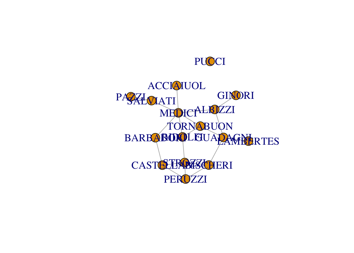
florence <- as.matrix(florence) # coerce into a matrix
florence <- graph.adjacency(florence, mode = "undirected", diag = FALSE)

plot(florence) # plot the graph
degree(florence)
## ACCIAIUOL   ALBIZZI BARBADORI  BISCHERI CASTELLAN    GINORI  GUADAGNI
##         1         3         2         3         3         1         4
## LAMBERTES    MEDICI     PAZZI   PERUZZI     PUCCI   RIDOLFI  SALVIATI
##         1         6         1         3         0         3         2
##   STROZZI TORNABUON
##         4         3
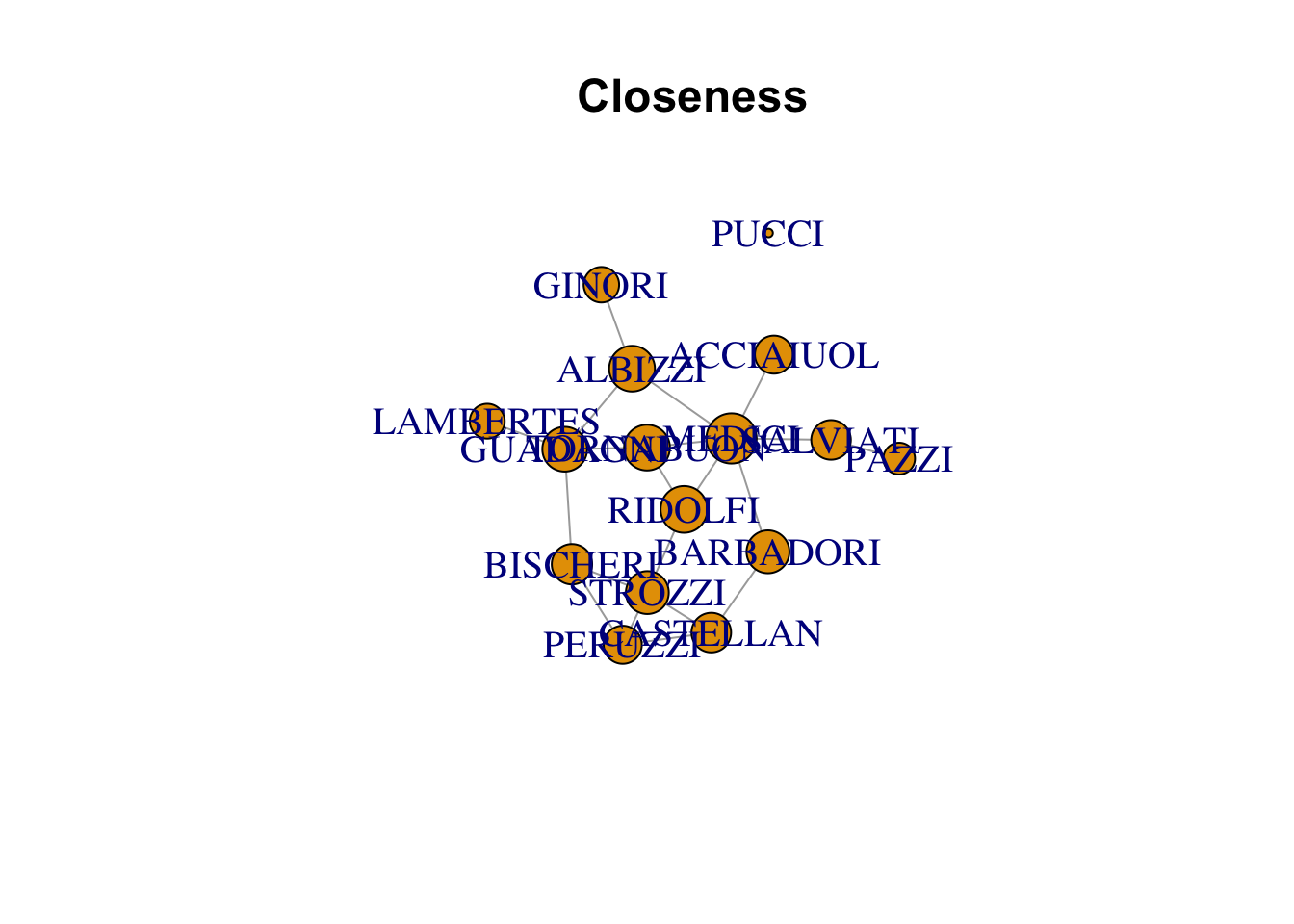
closeness(florence)
##   ACCIAIUOL     ALBIZZI   BARBADORI    BISCHERI   CASTELLAN      GINORI
## 0.018518519 0.022222222 0.020833333 0.019607843 0.019230769 0.017241379
##    GUADAGNI   LAMBERTES      MEDICI       PAZZI     PERUZZI       PUCCI
## 0.021739130 0.016949153 0.024390244 0.015384615 0.018518519 0.004166667
##     RIDOLFI    SALVIATI     STROZZI   TORNABUON
## 0.022727273 0.019230769 0.020833333 0.022222222
1 / (closeness(florence) * 15)
## ACCIAIUOL   ALBIZZI BARBADORI  BISCHERI CASTELLAN    GINORI  GUADAGNI
##  3.600000  3.000000  3.200000  3.400000  3.466667  3.866667  3.066667
## LAMBERTES    MEDICI     PAZZI   PERUZZI     PUCCI   RIDOLFI  SALVIATI
##  3.933333  2.733333  4.333333  3.600000 16.000000  2.933333  3.466667
##   STROZZI TORNABUON
##  3.200000  3.000000
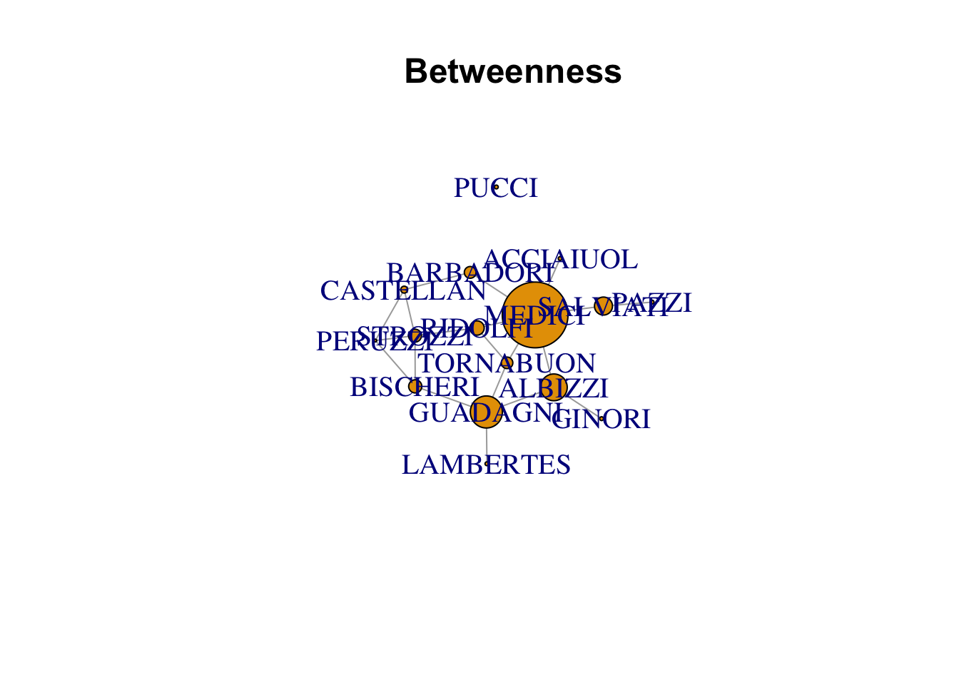
betweenness(florence)
## ACCIAIUOL   ALBIZZI BARBADORI  BISCHERI CASTELLAN    GINORI  GUADAGNI
##  0.000000 19.333333  8.500000  9.500000  5.000000  0.000000 23.166667
## LAMBERTES    MEDICI     PAZZI   PERUZZI     PUCCI   RIDOLFI  SALVIATI
##  0.000000 47.500000  0.000000  2.000000  0.000000 10.333333 13.000000
##   STROZZI TORNABUON
##  9.333333  8.333333
par(cex = 1.25)
plot(florence, vertex.size = closeness(florence) * 1000,
     main = "Closeness")
plot(florence, vertex.size = betweenness(florence),
     main = "Betweenness")
Section 5.2.4: Directed Graph and Centrality
twitter.senator$indegree <- degree(twitter.adj, mode = "in")
twitter.senator$outdegree <- degree(twitter.adj, mode = "out")

in.order <- order(twitter.senator$indegree, decreasing = TRUE)
out.order <- order(twitter.senator$outdegree, decreasing = TRUE)

## 3 greatest indegree
twitter.senator[in.order[1:3], ]
##       screen_name          name party state indegree outdegree
## 5     SenatorBurr  Richard Burr     R    NC        2         0
## 7     JohnBoozman  John Boozman     R    AR        2         0
## 8 SenJohnBarrasso John Barrasso     R    WY        2         0
## 3 greatest outdegree
twitter.senator[out.order[1:3], ]
##    screen_name            name party state indegree outdegree
## 2     RoyBlunt       Roy Blunt     R    MO        1        46
## 1 SenAlexander Lamar Alexander     R    TN        1        38
## 3 SenatorBoxer   Barbara Boxer     D    CA        0         7
n <- nrow(twitter.senator)
## color: Democrats = `blue', Republicans = `red', Independent = `black'
col <- rep("red", n)
col[twitter.senator$party == "D"] <- "blue"
col[twitter.senator$party == "I"] <- "black"
## pch: Democrats = circle, Republicans = diamond, Independent = cross
pch <- rep(16, n)
pch[twitter.senator$party == "D"] <- 17
pch[twitter.senator$party == "I"] <- 4
par(cex = 1.25)
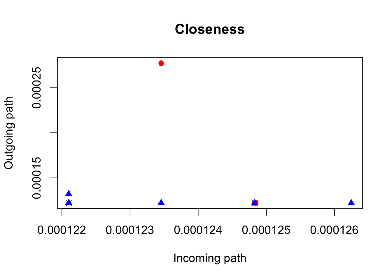
## plot for comparing two closeness measures (incoming vs. outgoing)
plot(closeness(twitter.adj, mode = "in"),
closeness(twitter.adj, mode = "out"), pch = pch, col = col,
main = "Closeness", xlab = "Incoming path", ylab = "Outgoing path")
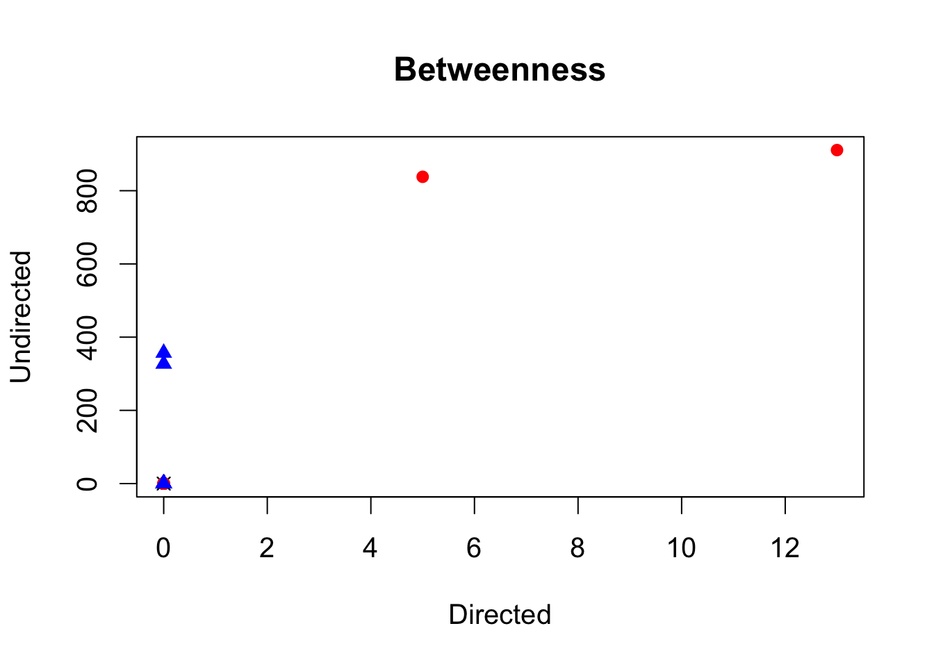
## plot for comparing directed and undirected betweenness
plot(betweenness(twitter.adj, directed = TRUE),
     betweenness(twitter.adj, directed = FALSE), pch = pch, col = col,
     main = "Betweenness", xlab = "Directed", ylab = "Undirected")
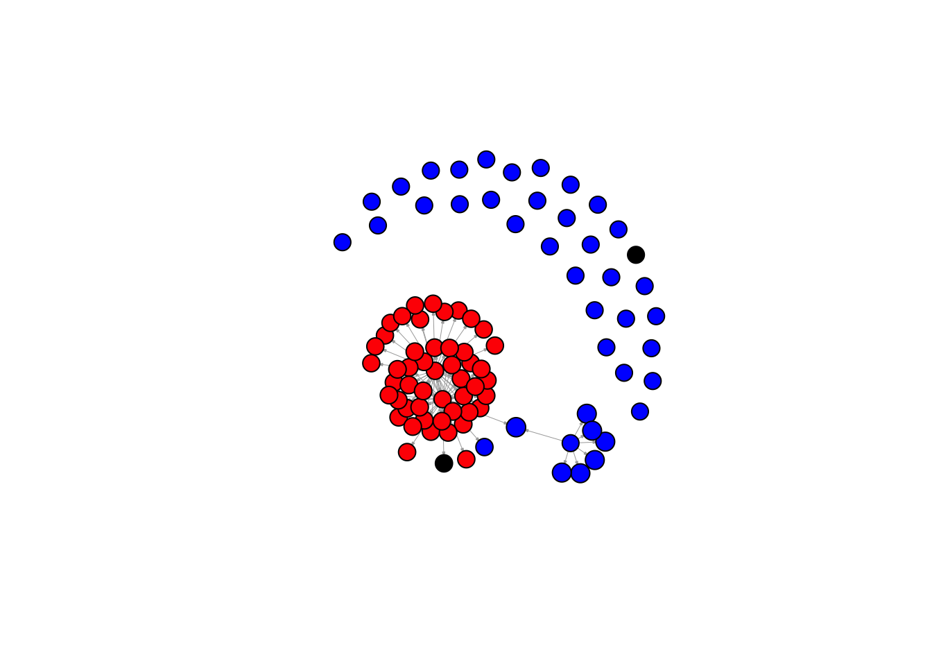
twitter.senator$pagerank <- page.rank(twitter.adj)$vector

par(cex = 1.25)
## `col' parameter is defined earlier
plot(twitter.adj, vertex.size = twitter.senator$pagerank * 1000,
     vertex.color = col, vertex.label = NA,
     edge.arrow.size = 0.1, edge.width = 0.5)

PageRank <- function(n, A, d, pr) { # function takes 4 inputs
    deg <- degree(A, mode = "out") # outdegree calculation
    for (j in 1:n) {
        pr[j] <- (1 - d) / n +  d * sum(A[ ,j] * pr / deg)
    }
    return(pr)
}

nodes <- 4

## adjacency matrix with arbitrary values
adj <- matrix(c(0, 1, 0, 1, 1, 0, 1, 0, 0, 1, 0, 0, 0, 1, 0, 0),
              ncol = nodes, nrow = nodes, byrow = TRUE)
adj
##      [,1] [,2] [,3] [,4]
## [1,]    0    1    0    1
## [2,]    1    0    1    0
## [3,]    0    1    0    0
## [4,]    0    1    0    0
adj <- graph.adjacency(adj)  # turn it into an igraph object

d <- 0.85  # typical choice of constant
pr <- rep(1 / nodes, nodes) # starting values

## maximum absolute difference; use a value greater than threshold
diff <- 100

## while loop with 0.001 being the threshold
while (diff > 0.001) {
    pr.pre <- pr # save the previous iteration
    pr <- PageRank(n = nodes, A = adj, d = d, pr = pr)
    diff <- max(abs(pr - pr.pre))
}
pr
## [1] 0.2213090 0.4316623 0.2209565 0.1315563
Section 5.3: Spatial Data
Section 5.3.1: The 1854 Cholera Outbreak in Action
Section 5.3.2: Spatial Data in R
library(maps)
data(us.cities)
head(us.cities)
##         name country.etc    pop   lat    long capital
## 1 Abilene TX          TX 113888 32.45  -99.74       0
## 2   Akron OH          OH 206634 41.08  -81.52       0
## 3 Alameda CA          CA  70069 37.77 -122.26       0
## 4  Albany GA          GA  75510 31.58  -84.18       0
## 5  Albany NY          NY  93576 42.67  -73.80       2
## 6  Albany OR          OR  45535 44.62 -123.09       0
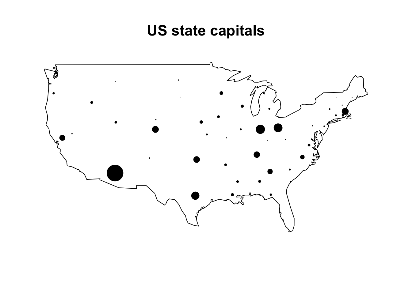
par(cex = 1.25)

map(database = "usa")
capitals <- subset(us.cities, capital == 2) # subset state capitals

## add points proportional to population using latitude and longitude
points(x = capitals$long, y = capitals$lat,
       cex = capitals$pop / 500000, pch = 19)
title("US state capitals") # add a title
par(cex = 1.25)
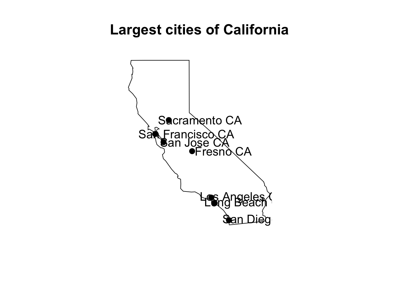
map(database = "state", regions = "California")
cal.cities <- subset(us.cities, subset = (country.etc == "CA"))
sind <- order(cal.cities$pop, decreasing = TRUE) # order by population
top7 <- sind[1:7] # seven cities with largest population
map(database = "state", regions = "California")
points(x = cal.cities$long[top7], y = cal.cities$lat[top7], pch = 19)
## add a constant to latitude to avoid overlapping with circles
text(x = cal.cities$long[top7] + 2.25, y = cal.cities$lat[top7],
label = cal.cities$name[top7])
title("Largest cities of California")
usa <- map(database = "usa", plot = FALSE) # save map
names(usa)  # list elements
## [1] "x" "y" "range" "names"
length(usa$x)
## [1] 7252
head(cbind(usa$x, usa$y)) # first five coordinates of a polygon
##           [,1]     [,2]
## [1,] -101.4078 29.74224
## [2,] -101.3906 29.74224
## [3,] -101.3620 29.65056
## [4,] -101.3505 29.63911
## [5,] -101.3219 29.63338
## [6,] -101.3047 29.64484
Section 5.3.3: Colors in R
allcolors <- colors()

head(allcolors)   # some colors
## [1] "white"         "aliceblue"     "antiquewhite"  "antiquewhite1"
## [5] "antiquewhite2" "antiquewhite3"
length(allcolors) # number of color names
## [1] 657
red <- rgb(red = 1, green = 0, blue = 0) # red
green <- rgb(red = 0, green = 1, blue = 0) # green
blue <- rgb(red = 0, green = 0, blue = 1) # blue
c(red, green, blue) # results
## [1] "#FF0000" "#00FF00" "#0000FF"
black <- rgb(red = 0, green = 0, blue = 0) # black
white <- rgb(red = 1, green = 1, blue = 1) # white
c(black, white) # results
## [1] "#000000" "#FFFFFF"
rgb(red = c(0.5, 1), green = c(0, 1), blue = c(0.5, 0))
## [1] "#800080" "#FFFF00"
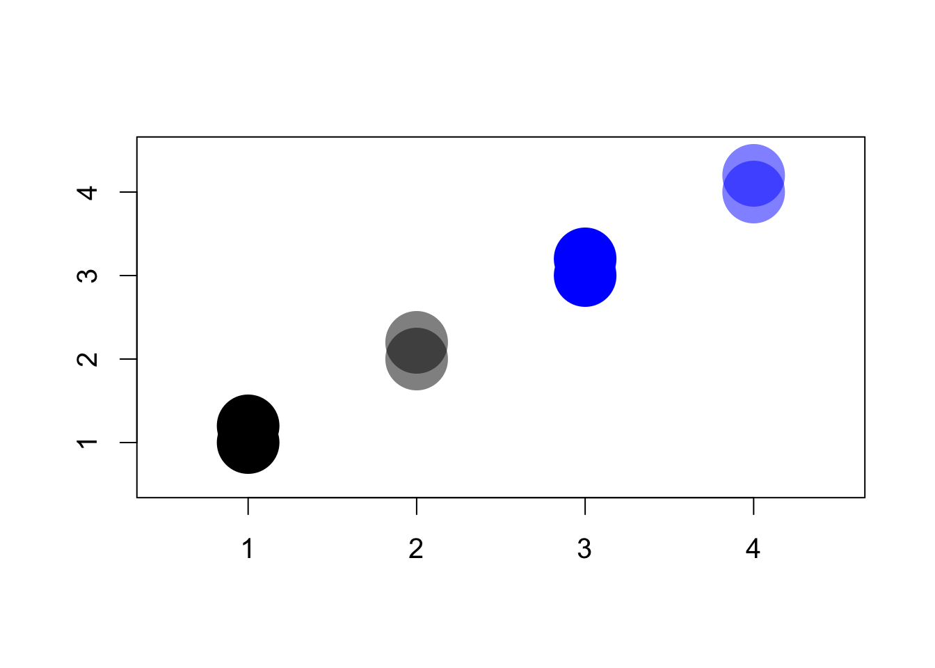
## semi-transparent blue
blue.trans <- rgb(red = 0, green = 0, blue = 1, alpha = 0.5)

## semi-transparent black
black.trans <- rgb(red = 0, green = 0, blue = 0, alpha = 0.5)

par(cex = 1.25)

## completely colored dots; difficult to distinguish
plot(x = c(1, 1), y = c(1, 1.2), xlim = c(0.5, 4.5), ylim = c(0.5, 4.5),
     pch = 16, cex = 5, ann = FALSE, col = black)
points(x = c(3, 3), y = c(3, 3.2), pch = 16, cex = 5, col = blue)

## semi-transparent; easy to distinguish
points(x = c(2, 2), y = c(2, 2.2), pch = 16, cex = 5, col = black.trans)
points(x = c(4, 4), y = c(4, 4.2), pch = 16, cex = 5, col = blue.trans)
Section 5.3.4: US Presidential Elections
data("pres08", package = "qss")
## two-party vote share
pres08$Dem <- pres08$Obama / (pres08$Obama + pres08$McCain)
pres08$Rep <- pres08$McCain / (pres08$Obama + pres08$McCain)

## color for California
cal.color <- rgb(red = pres08$Rep[pres08$state == "CA"],
                 blue = pres08$Dem[pres08$state == "CA"],
                 green = 0)

par(cex = 1.25)
## California as a blue state
map(database = "state", regions = "California", col = "blue",
    fill = TRUE)

## California as a purple state
map(database = "state", regions = "California", col = cal.color,
    fill = TRUE)

par(cex = 1.25)
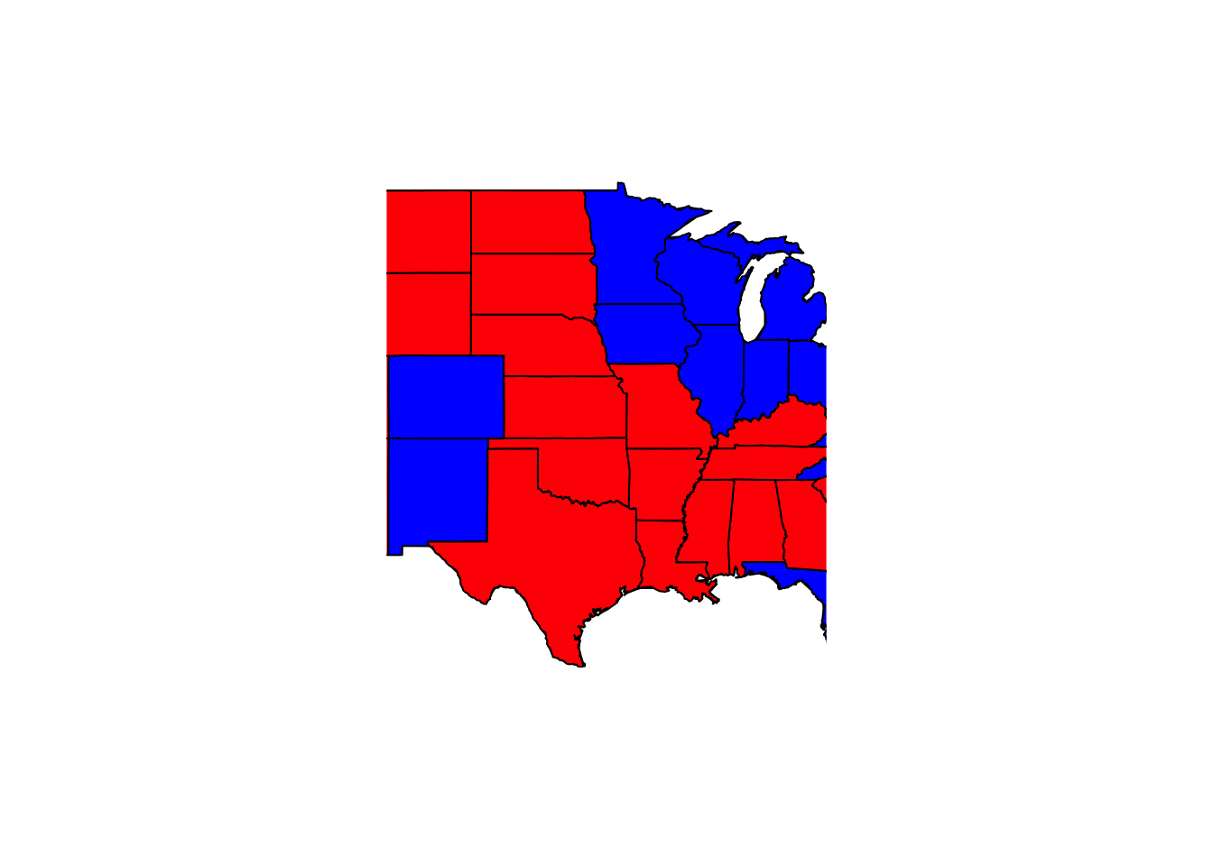
## America as red and blue states
map(database = "state") # create a map
for (i in 1:nrow(pres08)) {
if ((pres08$state[i] != "HI") & (pres08$state[i] != "AK") &
(pres08$state[i] != "DC")) {
map(database = "state", regions = pres08$state.name[i],
col = ifelse(pres08$Rep[i] > pres08$Dem[i], "red", "blue"),
fill = TRUE, add = TRUE)
}
}
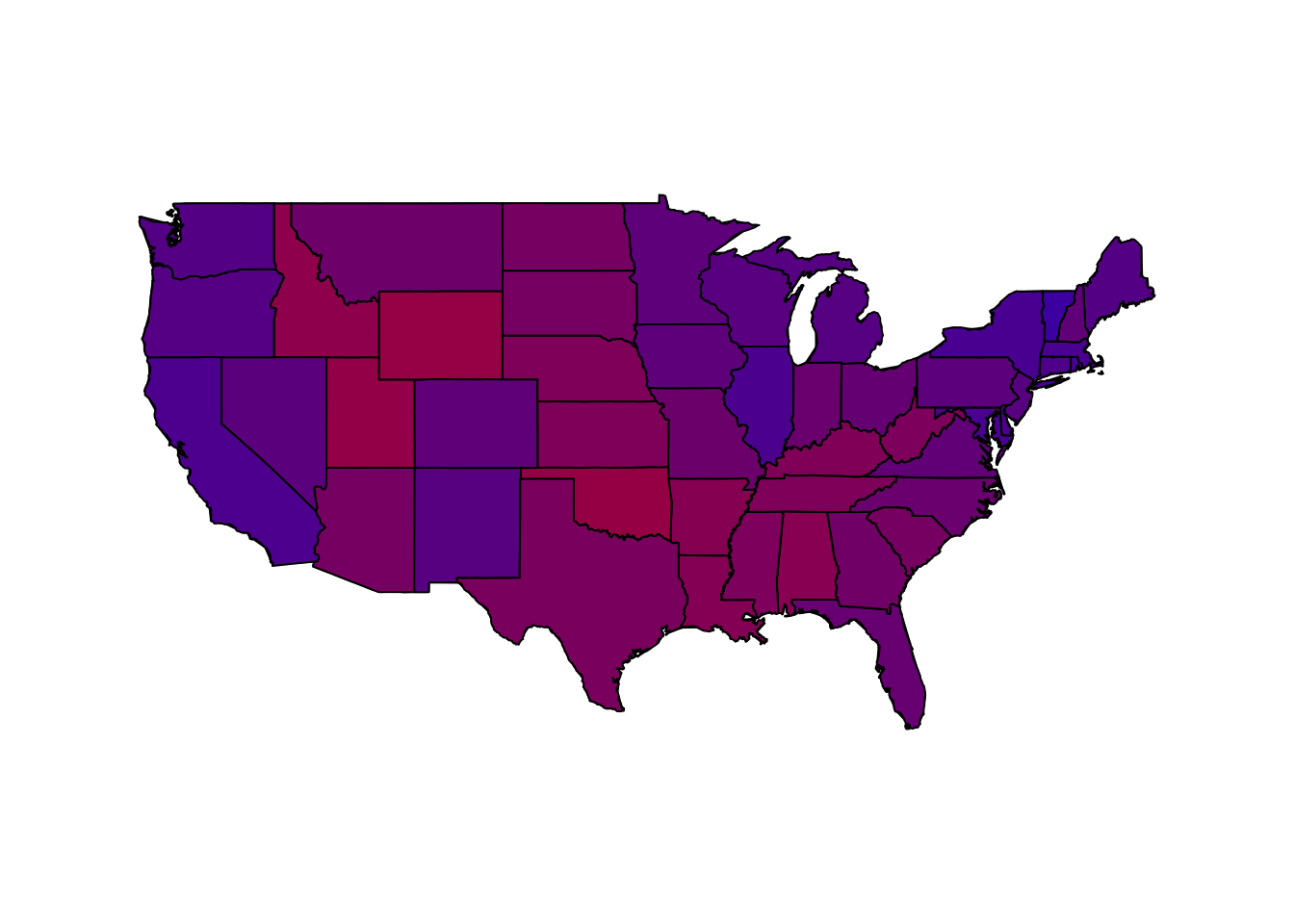
## America as purple states
map(database = "state") # create a map
for (i in 1:nrow(pres08)) {
    if ((pres08$state[i] != "HI") & (pres08$state[i] != "AK") &
        (pres08$state[i] != "DC")) {
        map(database = "state", regions = pres08$state.name[i],
            col = rgb(red = pres08$Rep[i], blue = pres08$Dem[i],
                green = 0), fill = TRUE, add = TRUE)
    }
}
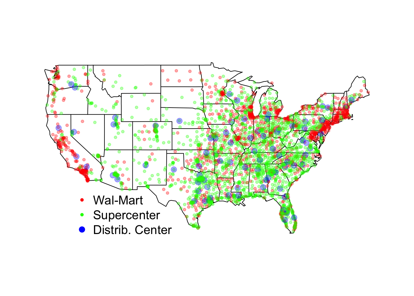
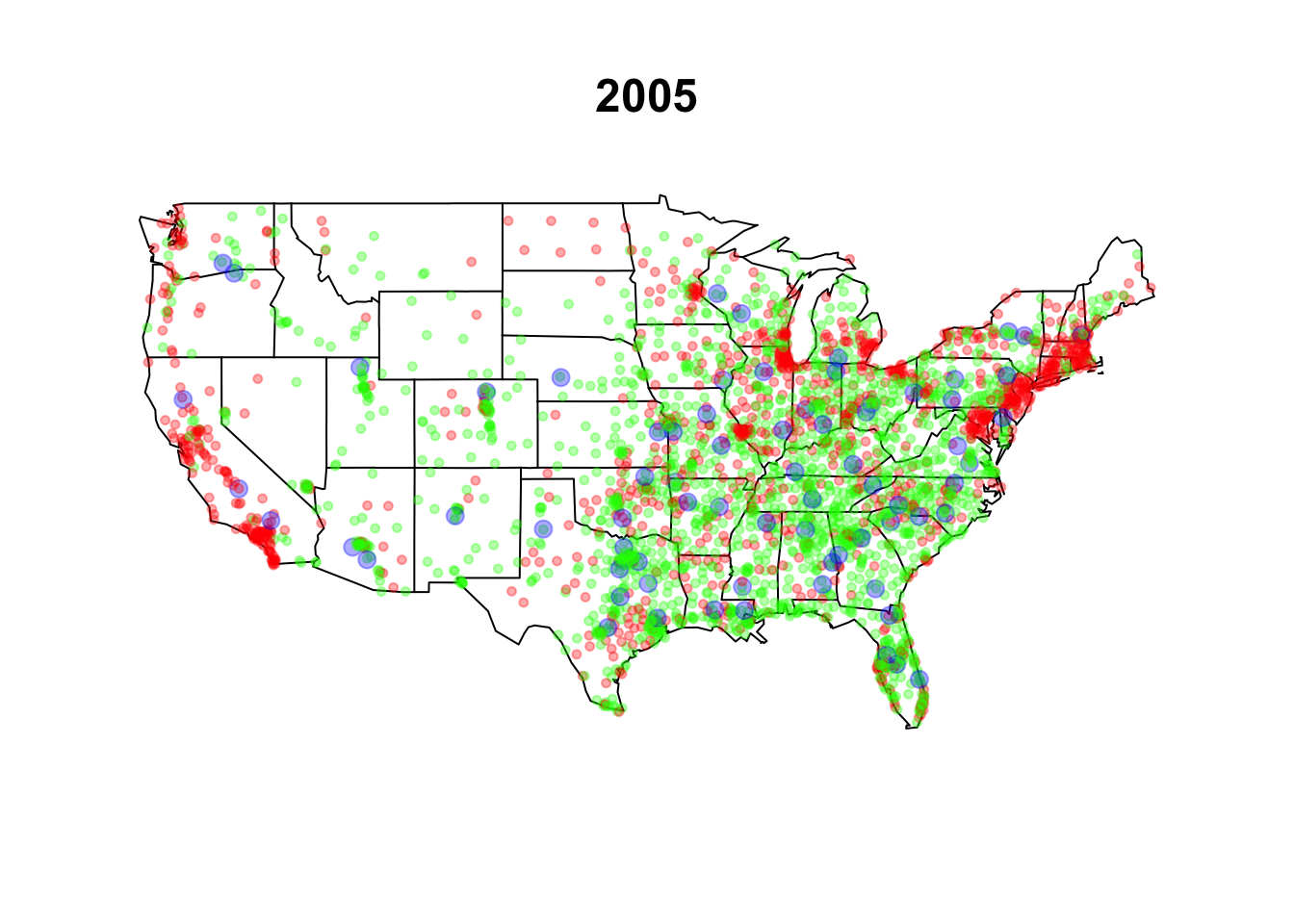
Section 5.3.5: Expansion of Walmart
data("walmart", package = "qss")

## red = WalMartStore, green = SuperCenter, blue = DistributionCenter
walmart$storecolors <- NA # create an empty vector

walmart$storecolors[walmart$type == "Wal-MartStore"] <-
    rgb(red = 1, green = 0, blue = 0, alpha = 1/3)
walmart$storecolors[walmart$type == "SuperCenter"] <-
    rgb(red = 0, green = 1, blue = 0, alpha = 1/3)
walmart$storecolors[walmart$type == "DistributionCenter"] <-
    rgb(red = 0, green = 0, blue = 1, alpha = 1/3)

## larger circles for DistributionCenter
walmart$storesize <- ifelse(walmart$type == "DistributionCenter", 1, 0.5)

par(cex = 1.25)
## map with legend
map(database = "state")

points(walmart$long, walmart$lat, col = walmart$storecolors,
       pch = 19, cex = walmart$storesize)

legend(x = -120, y = 32, bty = "n",
       legend = c("Wal-Mart", "Supercenter", "Distrib. Center"),
       col = c("red", "green", "blue"), pch = 19, # solid circles
       pt.cex = c(0.5, 0.5, 1)) # size of circles
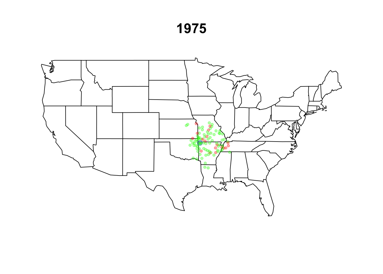
Section 5.3.6: Animation in R
walmart.map <- function(data, date) {
    walmart <- subset(data, subset = (opendate <= date))
    map(database = "state")
    points(walmart$long, walmart$lat, col = walmart$storecolors,
           pch = 19, cex = walmart$storesize)
}

par(cex = 1.25)

walmart$opendate <- as.Date(walmart$opendate)

walmart.map(walmart, as.Date("1974-12-31"))
title("1975")
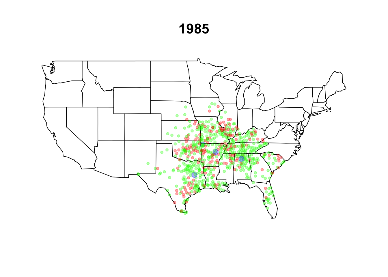
walmart.map(walmart, as.Date("1984-12-31"))
title("1985")
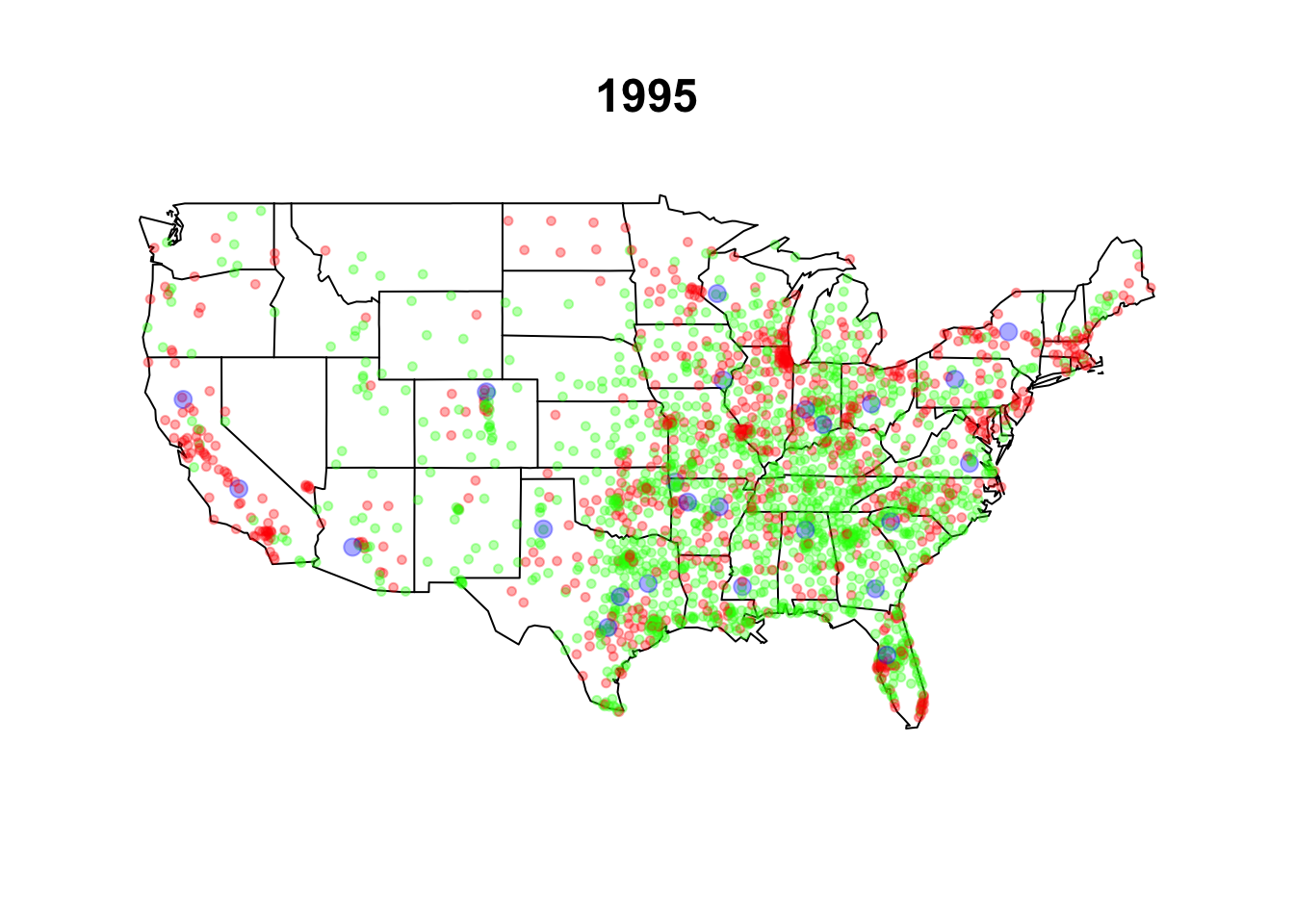
walmart.map(walmart, as.Date("1994-12-31"))
title("1995")
walmart.map(walmart, as.Date("2004-12-31"))
title("2005")
n <- 25 # number of maps to animate
dates <- seq(from = min(walmart$opendate),
             to = max(walmart$opendate), length.out = n)
## library("animation")
## saveHTML({
##     for (i in 1:length(dates)) {
##         walmart.map(walmart, dates[i])
##         title(dates[i])
##     }
## }, title = "Expansion of Walmart", htmlfile = "walmart.html",
##          outdir = getwd(), autobrowse = FALSE)